Descriptive Statistics — Part I: Summarising Numeric Variables

Before you begin, take a few minutes to check what you already know and how confident you feel. You will see the same questions again at the end of the module — this helps both you and us measure what you have learned. Click an option for every question and confidence rating, then click Next to continue.

In Module 2 you learned to reshape and filter a dataset with dplyr verbs. Now you have a clean column of patient values — ages, BMIs, CRP results — and your reader wants the headline. Descriptive statistics is how you turn a column of numbers into the one or two figures that go in a table or the first line of a results paragraph.

This part of the module covers three foundations for summarising a numeric variable:

• Location — the mean, median, and mode, and choosing which one represents the typical patient.
• Spread — the standard deviation, variance, IQR, and range, and which spread number pairs with which centre.
• Shape and skew — spotting when a right-tailed lab pulls the mean away from the median, and switching to median (IQR).

By the end of this part you will be able to summarise a numeric variable with the right centre-and-spread pair, explain why the median and IQR resist a single extreme value while the mean and SD are dragged by it, and recognise a right-skewed lab from the mean-versus-median gap and report median (IQR) instead of mean (SD).

Try every snippet in the R Scratchpad on the right. The dataset patients.csv is already loaded for the centre-and-spread examples, and you will build a small right-skewed CRP cohort with set.seed() so your numbers match the lesson exactly.

A measure of location is a single number that stands in for a whole column — the value a typical patient sits near. The three you will use are the mean, the median, and the mode.

The mean is the arithmetic average: add every value, divide by how many there are. You compute it with mean(). For five ages c(10, 12, 14, 16, 18), the mean is 14.

ages <- c(54, 61, 47, 73, 58)
mean(ages)

The median is the middle value once the numbers are sorted: half the patients fall below it, half above. You compute it with median(). The median barely moves when one value is extreme, which is why it is the safer centre for lab results.

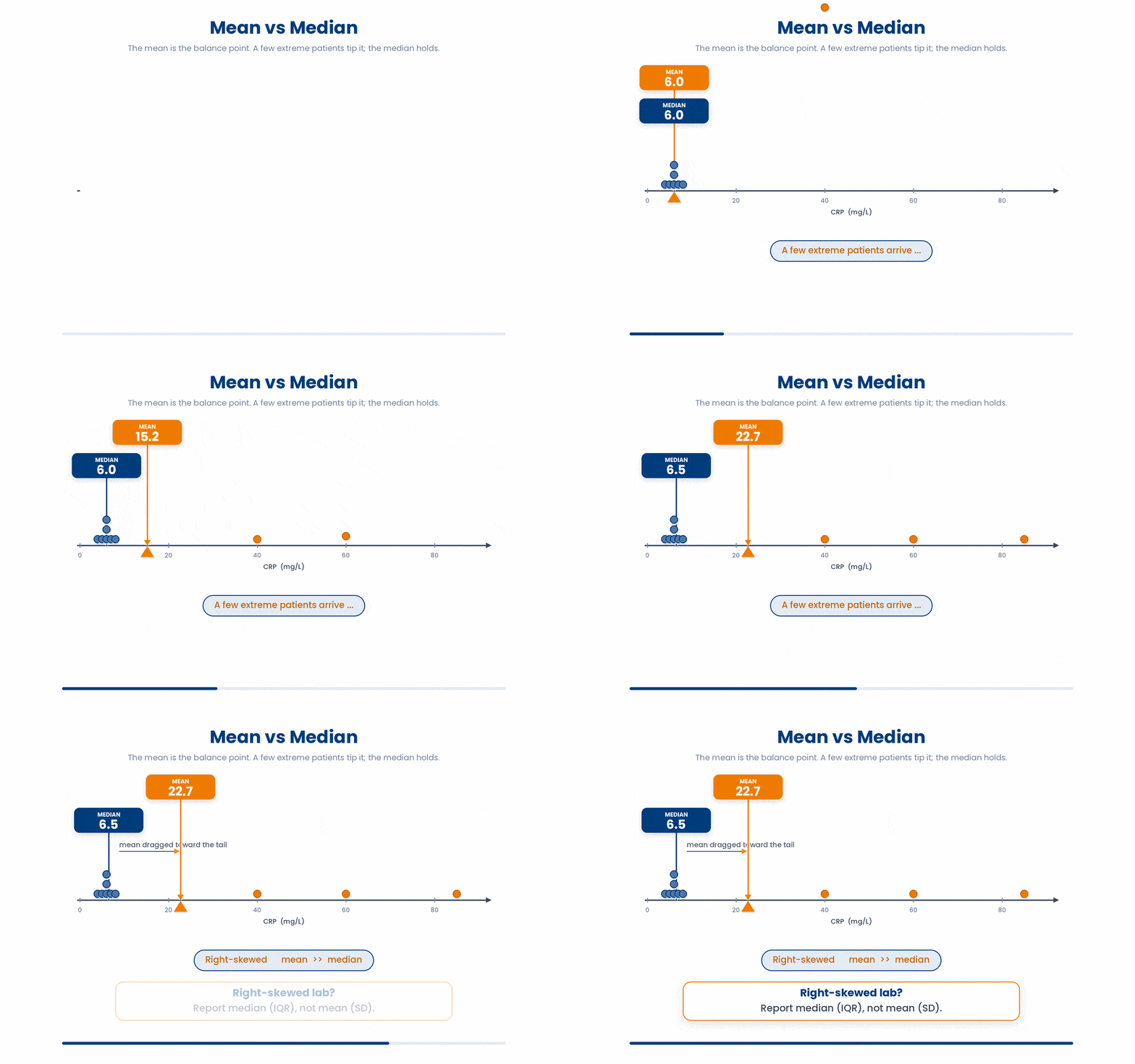
Watch what one extreme value does. The median of c(2, 4, 9, 100) is the average of the two middle numbers, 4 and 9 — so 6.5. That single 100 leaves the median almost untouched, but it would drag the mean up past 28.

median(c(2, 4, 9, 100))

The mode is the most frequent value. It is the only centre that makes sense for a category — the most common treatment arm, the commonest diagnosis. R has no built-in mode() for this (that name means something else), so for a category you read the mode off a count table, which you will build later in this part.

Here is the classic trap. R has a function called mode(), but it returns the storage type of an object, not the most common value. Calling mode(c(1, 1, 2)) gives "numeric", not 1. R does not have a standard built-in function to calculate the statistical mode

A centre alone is never enough. Two wards can share a mean HbA1c of 7.5 yet look completely different — one tightly clustered, one swinging from 5 to 11. A measure of spread tells you how scattered the values are around that centre.

The standard deviation (SD) is the typical distance of a value from the mean, in the original units. You compute it with sd(). A small SD means patients cluster near the mean; a large SD means they are spread wide.

The variance is simply the SD squared, computed with var(). It lives in squared units, which is hard to interpret, so you report the SD in a table and keep the variance for the maths underneath.

hba1c <- c(7.2, 8.1, 6.5, 9.4, 7.8)
mean(hba1c)
sd(hba1c)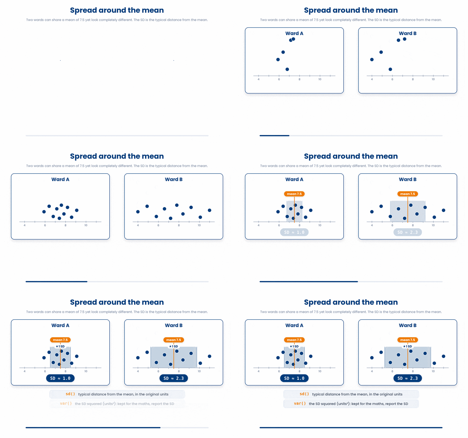

For the simple ages c(10, 20, 30), the variance is 100 and the SD is its square root, 10.

The range is the lowest and highest value. R's range() returns both as a pair, smallest first — so range(c(3, 9, 1)) gives 1 9. It flags outliers and data-entry errors fast, but a single typo of 999 for 99 blows it wide open, so never report the range as your only measure of spread.

hba1c <- c(7.2, 8.1, 6.5, 9.4, 7.8)
range(hba1c)

The interquartile range (IQR) is the spread of the middle half of the data: the distance from the 25th percentile up to the 75th. You compute it with IQR(). Like the median, it shrugs off extreme values, so it is the spread you pair with a median. For c(1, 2, 3, 4, 5) the IQR is 2.

hba1c <- c(7.2, 8.1, 6.5, 9.4, 7.8)
IQR(hba1c)

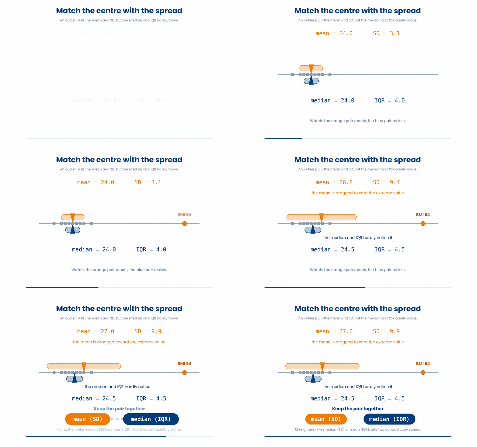
Centre and spread come as matched pairs. Report the mean with the SD — written mean (SD) — because both are pulled the same way by extreme values. Report the median with the IQR — written median (IQR) — because both resist extreme values.

library(readr)
patients <- read_csv("patients.csv")
mean(patients$bmi)
sd(patients$bmi)
median(patients$bmi)
IQR(patients$bmi)

The mismatched trap is to report the median with the SD, or the mean with the IQR. Mixing a resistant centre with a non-resistant spread tells your reader two contradictory stories about the same column. Keep the pairs together: mean (SD), or median (IQR).

The pairing rule has a deeper reason behind it: the shape of the data. When values are roughly symmetric around the centre — like adult height — the mean and median nearly agree, and mean (SD) is honest.

Many clinical labs are not symmetric. They are right-skewed: most patients sit low, but a long tail of high values stretches to the right. C-reactive protein (CRP), triglycerides, and hospital length-of-stay all behave this way — a few very sick patients sit far out in the tail.

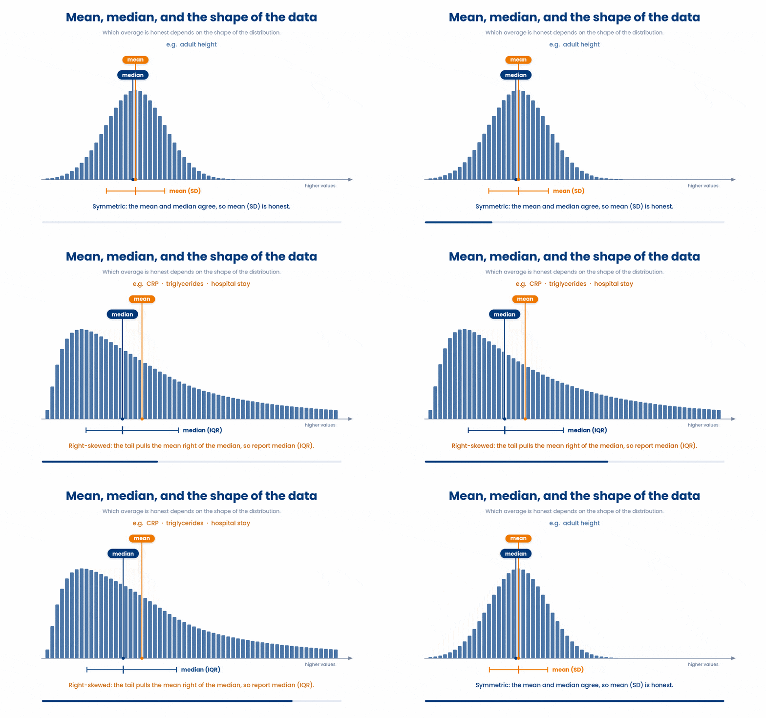
In a right-skewed variable, that tail drags the mean upward but leaves the median in place. So the mean lands above the median, and reporting the mean would overstate the typical patient. The rule of thumb: when the mean and median diverge noticeably, report the median (IQR).

Build a right-skewed CRP cohort and see the gap for yourself. The set.seed() line fixes the random draw so your numbers match this lesson exactly.

set.seed(42)
crp <- round(rexp(200, rate = 0.2), 1)
mean(crp)
median(crp)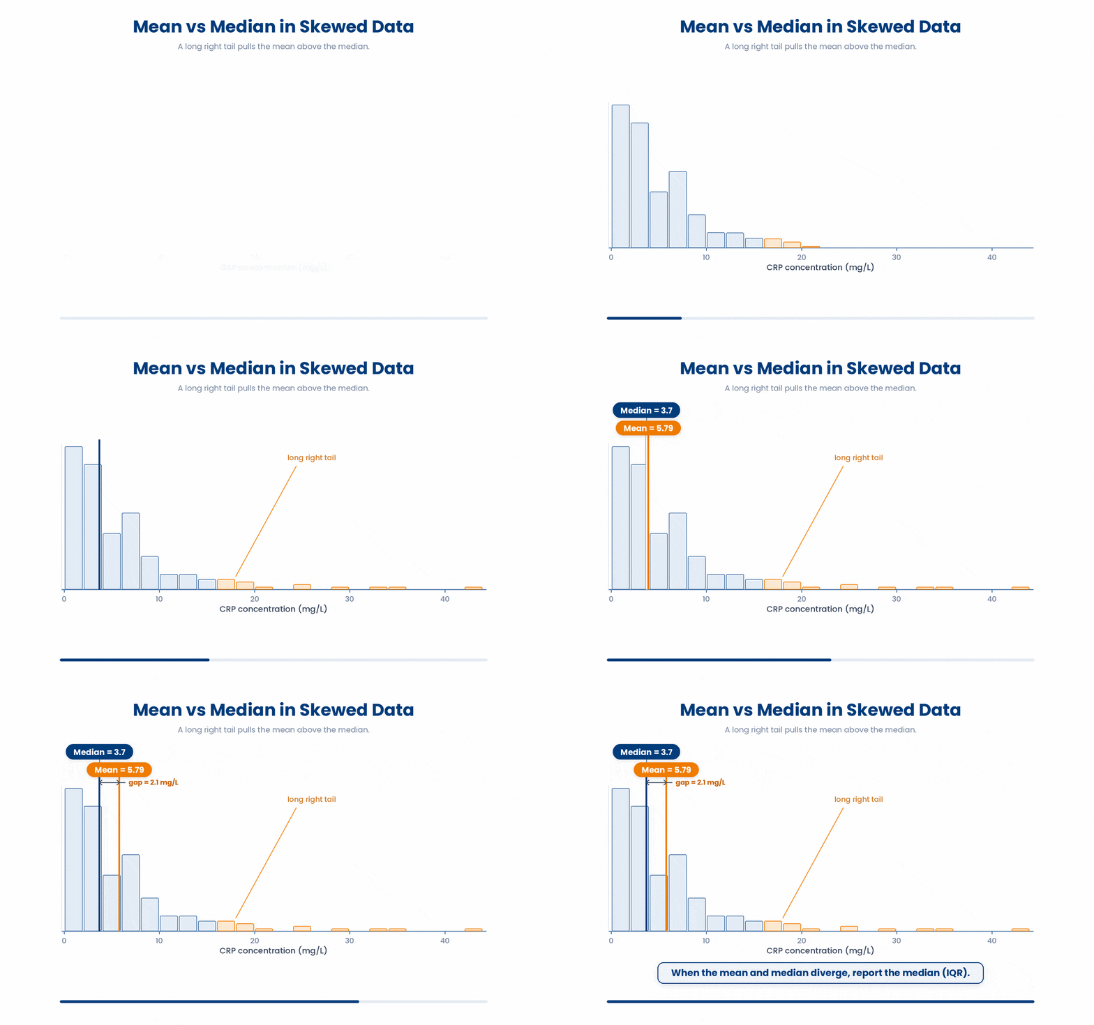

The mean comes out clearly above the median — the signature of right skew. A histogram makes the long right tail obvious; a ggplot must be printed at the top level to render, so just name the plot object or call it directly.

set.seed(42)
crp <- round(rexp(200, rate = 0.2), 1)
library(ggplot2)
ggplot(data.frame(crp = crp), aes(x = crp)) +
  geom_histogram(bins = 30) +
  labs(x = "CRP (mg/L)", y = "Patients")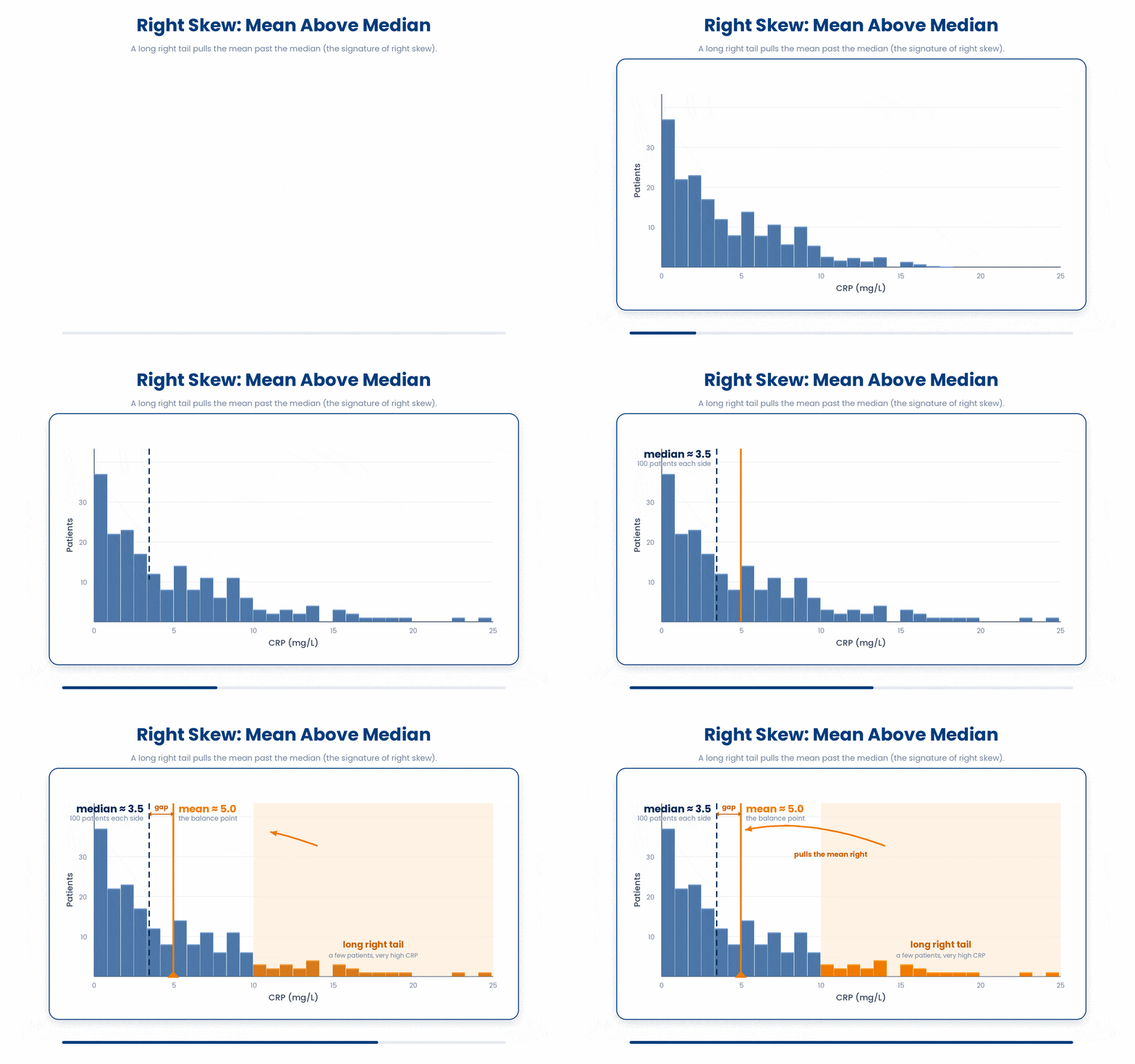

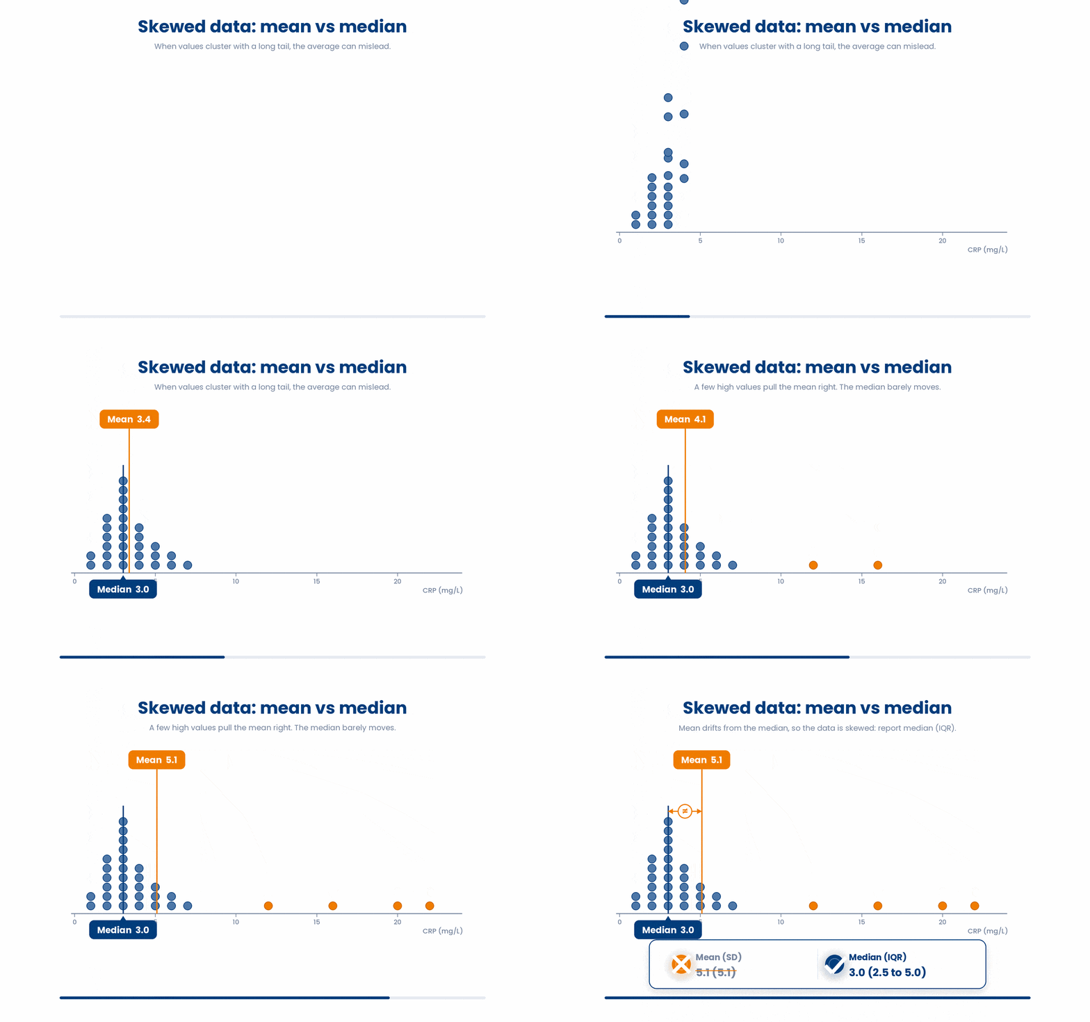
The novice trap is to report mean (SD) for an obviously skewed value — an average CRP of, say, 5.1 mg/L when most patients sit near 3. The right way: glance at the mean-versus-median gap (or a quick histogram), and if the variable is skewed, switch to median (IQR).

You have reached the end of the module. Try the same questions again — your answers here, paired with your pre-test answers, are how we measure what the module taught you. Answer every question and confidence rating, then click Submit and see results to view your score.

Here is how your post-test answers compare with your pre-test answers. The pre/post pairing is the most reliable way to see what this module actually taught you.