

1 Before you start
This is not graded, and it does not count towards anything. Answer every question even if you are only guessing — having a go at something before you have been taught it is one of the best ways to remember it afterwards. The lesson ends with another short check, and there you will be shown the correct answer for anything you missed. Choose an option for every question and confidence rating, then click Submit answers.
Your data has one row per patient with columns visit_1 and visit_2 holding HbA1c. A model needs one row per measurement with a single hba1c column. Which function reshapes it?
Which function turns a long table back into a wide one, with more columns and fewer rows?
In pivot_longer(cols = c(visit_1, visit_2), names_to = "visit", values_to = "hba1c"), what does names_to control?
Before clean_names() you had to write df$`Patient ID` with backticks, but after it you write df$patient_id with none. Why do the backticks become unnecessary?
You leave treatment as plain text ("Drug", "Placebo") and fit a model. Which arm does R pick as the reference, and how do you override it?
After arm <- fct_relevel(factor(c("Drug", "Placebo")), "Placebo"), what does levels(arm)[1] return, and why does it matter?
A spreadsheet recorded the placebo arm as "PBO" and you want the readable label "Placebo" without changing which level is the reference. Which call does this?
After you run clean_names() on a table, the column Patient ID becomes which tidy name?
I can reshape a clinical table between wide and long with pivot_longer() and pivot_wider(), and say which shape a plot or model needs.
I can set a factor's reference level with fct_relevel() before fitting a model, and rename messy level labels with fct_recode().
I can clean a messy spreadsheet's headers into tidy snake_case with clean_names() as the first step of an analysis.
2 Introduction
In Part III you combined two tables side by side with joins, matching rows on a shared key so no patient silently disappeared. Joins put tables next to each other; this part changes the shape of a single table and the way it reads a categorical variable. You will switch a table between wide and long, tell a model which group is the baseline it compares against, and clean the ugly column names a spreadsheet export hands you.
This part of the module covers three wrangling skills you reach for whenever real data meets a plot or a model:
- Pivots — reshape one table with pivot_longer() and pivot_wider() to move between wide and long, because ggplot2 and most models want one row per measurement.
- Factors and the reference level — set a factor's baseline group with fct_relevel() and rename messy labels with fct_recode(), so every model coefficient is compared against the group you chose, not the alphabetical default.
- Cleaning headers — rewrite ugly spreadsheet column names into tidy snake_case in one call with clean_names(), so you stop wrapping every reference in backticks.
By the end of this part you will be able to reshape data between wide and long with pivot_longer() and pivot_wider(), set a factor's reference level deliberately before you fit a model, and clean a messy export's headers as the first step of an analysis.
Try every snippet in the R Scratchpad on the right — the dataset diabetes_clinic.csv is already loaded, and you can build the small wide and messy tables yourself with tibble().
3 Wide and long: reshaping with pivots
Joins combine tables side by side; pivots change a single table's shape. The same data can be stored wide — one row per patient, with a separate column for each visit's HbA1c — or long — one row per measurement, with a visit column and a single hba1c value column. Wide is compact for a human to read; long is what ggplot2 and most models actually want.
Make a tiny wide table — three patients, HbA1c at two visits each:
Try this snippet in the R Scratchpad on the right.
library(tidyr)
wide <- tibble(
  patient_id = c("D001", "D002", "D003"),
  visit_1 = c(7.2, 8.1, 6.5),
  visit_2 = c(6.9, 7.8, 6.4)
)
wide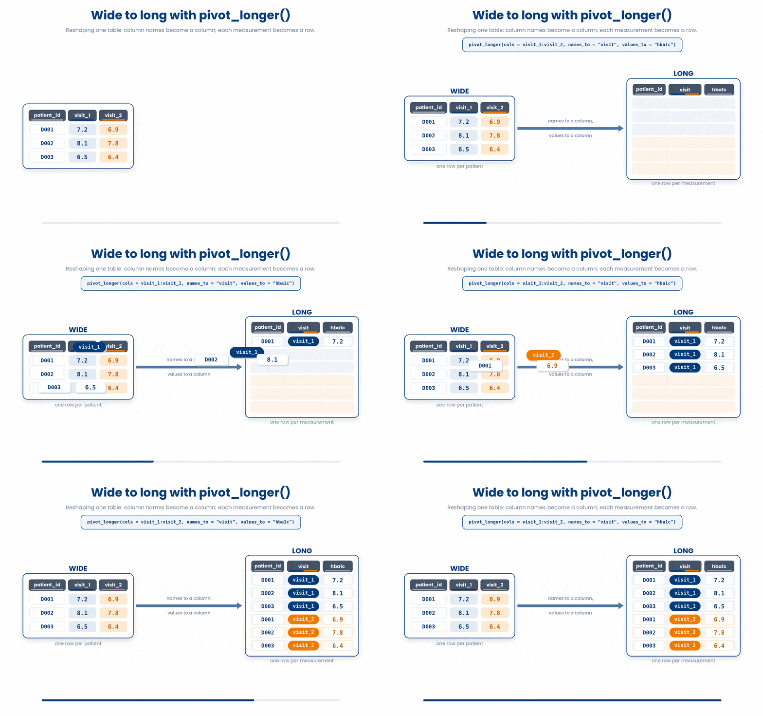
Use pivot_longer() to stack the visit columns into two new columns: one holding the old column names, one holding the values. You name them with names_to and values_to. The result has more rows and fewer columns — it grew longer.
Try this snippet in the R Scratchpad on the right.
library(tidyr)
wide <- tibble(
  patient_id = c("D001", "D002", "D003"),
  visit_1 = c(7.2, 8.1, 6.5),
  visit_2 = c(6.9, 7.8, 6.4)
)
long <- wide |>
  pivot_longer(
    cols = c(visit_1, visit_2),
    names_to = "visit",
    values_to = "hba1c"
  )
long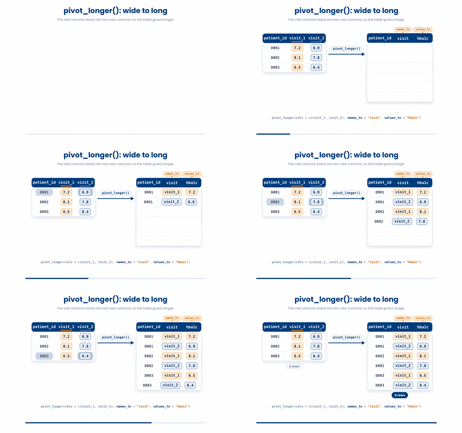
Use pivot_wider() to do the reverse: spread one column of names back out into separate columns. It is the inverse of pivot_longer().
Try this snippet in the R Scratchpad on the right.
library(tidyr)
wide <- tibble(
  patient_id = c("D001", "D002", "D003"),
  visit_1 = c(7.2, 8.1, 6.5),
  visit_2 = c(6.9, 7.8, 6.4)
)
long <- wide |>
  pivot_longer(c(visit_1, visit_2), names_to = "visit", values_to = "hba1c")
long |>
  pivot_wider(
    names_from = visit,
    values_from = hba1c
  )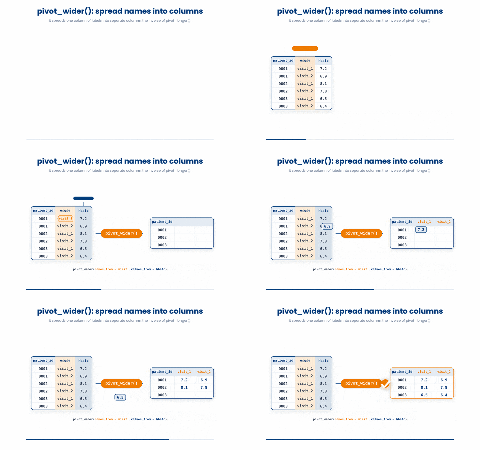
The trap is mixing up the direction. pivot_longer() goes wide-to-long; pivot_wider() goes long-to-wide. A memory hook: pivot_longer() makes the table longer (more rows), pivot_wider() makes it wider (more columns). When a plot or model complains it wants one row per observation, you almost always need pivot_longer().
4 Factors and the reference level
Reshaping is done; now you clean categories so a model reads them correctly. Recall from Part I that a factor is R's type for a category with a fixed set of allowed values, called its levels. The detail that matters for statistics is the first level: it is the reference level, the baseline that every other group is compared against in a model.
Concretely, when you regress an outcome on treatment, the model reports each arm's effect relative to the reference arm. If Placebo is the reference, the coefficient for Drug is the difference between Drug and Placebo — exactly the comparison you want. Choose the reference deliberately, because it changes what every coefficient means.
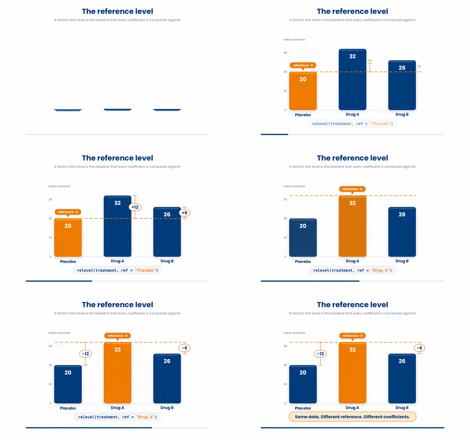
Here is the trap, and it is silent. If you leave the variable as plain text, R turns it into a factor for you and picks the reference alphabetically. "Drug" comes before "Placebo", so Drug becomes the baseline — and every odds ratio is now reported the wrong way round, with no error to warn you. Always make the variable a factor and set the reference yourself.
You set it with fct_relevel() from the forcats package, naming the level you want first. Build a vector and pull Placebo to the front:
Try this snippet in the R Scratchpad on the right.
library(forcats)
arm <- factor(c("Drug", "Placebo", "Drug", "Placebo"))
levels(arm)
arm <- fct_relevel(arm, "Placebo")
levels(arm)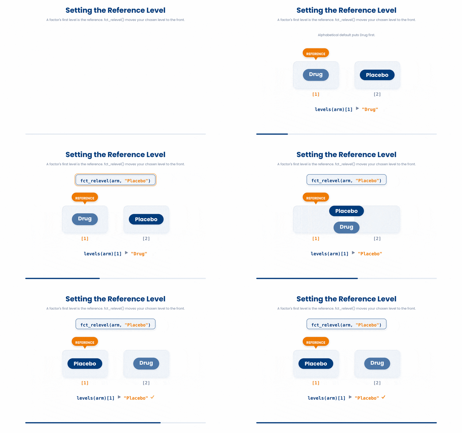
Before the relevel, levels(arm) lists Drug first — the alphabetical default. After fct_relevel(arm, "Placebo"), Placebo is first and becomes the reference. The first element of levels() is always the reference, so you can check your work by reading levels(arm)[1].
You can also rename messy level labels with fct_recode(), giving new = "old" pairs — useful when a spreadsheet recorded the placebo arm as "PBO" and you want a readable "Placebo".
Try this snippet in the R Scratchpad on the right.
raw_arm <- factor(c("PBO", "DRG", "PBO"))
tidy_arm <- fct_recode(raw_arm, Placebo = "PBO", Drug = "DRG")
levels(tidy_arm)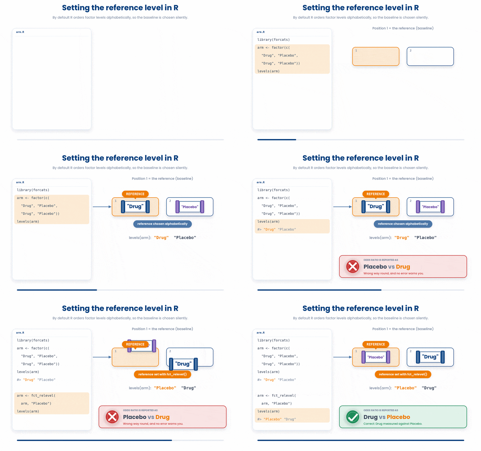
5 Cleaning messy spreadsheet headers
One more habit before you wrangle real exports. Spreadsheets arrive with ugly column names: spaces, capitals, and symbols like Patient ID or HbA1c (%). Names like that are awkward to type and force you to wrap every reference in backticks. The janitor package fixes them in one call.
clean_names() rewrites every column name into snake_case — lowercase words joined by underscores, with symbols stripped. Patient ID becomes patient_id, HbA1c (%) becomes hb_a1c. Consistent, lowercase, underscore-separated names are the tidyverse convention and save you constant backticking.
Try this snippet in the R Scratchpad on the right.
library(janitor)
library(tibble)
messy <- tibble(
  `Patient ID` = c("D001", "D002"),
  `Age (years)` = c(54, 61),
  `Treatment Arm` = c("Placebo", "Drug")
)
messy <- clean_names(messy)
names(messy)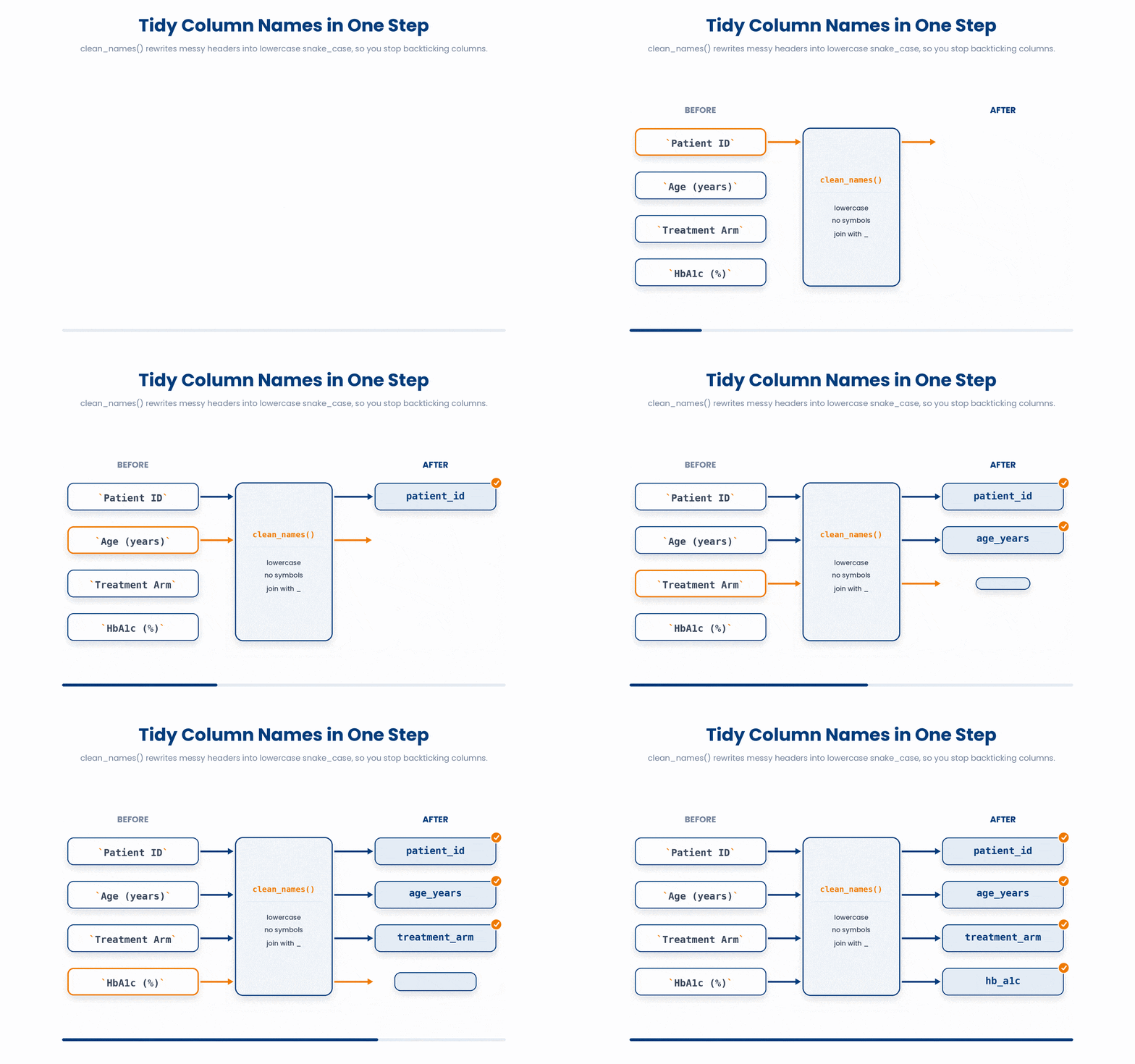
Make clean_names() the first thing you do after reading a messy file, before any select or mutate. Every later line then refers to tidy, predictable names instead of fragile backticked originals.
6 Put it together
This Parsons problem gives you the right lines in the wrong order, plus a few lines that do not belong. Drag the correct lines into order — you must build both tables before you can join them — and leave the wrong ones in the bank.
All the lines you need are in the Line bank on the left — some may be distractors you should leave behind. Drag the lines you need into the Your solution column on the right, in the correct order, then click Check.
Task: Build a demographics table and a labs table, then left_join() them on patient_id so every patient is kept. Each table must exist before the join runs.
labs <- tibble(patient_id = c("D001", "D001"), hba1c = c(7.2, 7.5))demographics <- tibble(patient_id = c("D001", "D002"), age = c(54, 61))left_join(labs)left_join(demographics, labs, by = "patient_id")demographics <- left_join(by = "patient_id")inner_join(demographics)
- Drop lines here, in order.
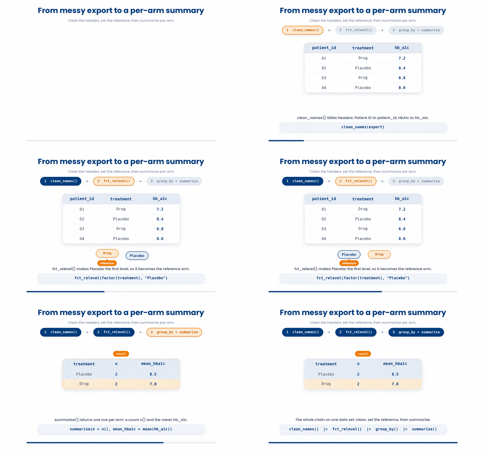
Now chain the moves end to end: clean a messy export, set Placebo as the reference, then summarise HbA1c per arm with a count. The worked example fades its support — first you study a full solution, then you fill the gaps, then you solve a fresh one on your own.
Work through this example in three stages. You unlock each stage only after the tutor confirms the previous one. Each stage removes more of the scaffolding — by the end you are writing it yourself.
Problem: A spreadsheet export has the columns Patient ID, Treatment, and HbA1c, with treatment recorded as Placebo or Drug. Clean the headers, make Placebo the reference level, then report the count and mean HbA1c per arm. (Steps are written as separate assignments here so the pipe symbol does not clash with the example format.)
library(dplyr)
library(janitor)
library(forcats)
export <- tibble(
  `Patient ID` = c("D1", "D2", "D3", "D4"),
  Treatment = c("Drug", "Placebo", "Drug", "Placebo"),
  HbA1c = c(7.2, 8.4, 6.8, 8.6)
)
export <- clean_names(export)
export <- mutate(export, treatment = fct_relevel(factor(treatment), "Placebo"))
grouped <- group_by(export, treatment)
summarise(grouped, n = n(), mean_hba1c = mean(hb_a1c, na.rm = TRUE))- clean_names() turns Patient ID into patient_id and HbA1c into hb_a1c (the capital A makes a word boundary)
- factor(treatment) makes the text a factor, then fct_relevel() pulls Placebo to the front as the reference
- group_by(export, treatment) splits the rows by arm
- summarise() returns one row per arm with its count n() and mean hba1c
The same solution with key parts replaced by ???.
Fill in every ??? so the code matches the reference,
then ask the tutor to check it.
Your turn: Now compute just one number from four HbA1c results (7.2, 8.1, 6.5, 9.4): store them in a vector called hba1c and report the mean, rounded to one decimal place.
7 Check your understanding
You have reached the end of the module. Try the same questions again — your answers here, paired with your pre-test answers, are how we measure what the module taught you. Answer every question and confidence rating, then click Submit and see results to view your score.
Your data has one row per patient with columns visit_1 and visit_2 holding HbA1c. A model needs one row per measurement with a single hba1c column. Which function reshapes it?
Which function turns a long table back into a wide one, with more columns and fewer rows?
In pivot_longer(cols = c(visit_1, visit_2), names_to = "visit", values_to = "hba1c"), what does names_to control?
Before clean_names() you had to write df$`Patient ID` with backticks, but after it you write df$patient_id with none. Why do the backticks become unnecessary?
You leave treatment as plain text ("Drug", "Placebo") and fit a model. Which arm does R pick as the reference, and how do you override it?
After arm <- fct_relevel(factor(c("Drug", "Placebo")), "Placebo"), what does levels(arm)[1] return, and why does it matter?
A spreadsheet recorded the placebo arm as "PBO" and you want the readable label "Placebo" without changing which level is the reference. Which call does this?
After you run clean_names() on a table, the column Patient ID becomes which tidy name?
I can reshape a clinical table between wide and long with pivot_longer() and pivot_wider(), and say which shape a plot or model needs.
I can set a factor's reference level with fct_relevel() before fitting a model, and rename messy level labels with fct_recode().
I can clean a messy spreadsheet's headers into tidy snake_case with clean_names() as the first step of an analysis.
8 Your results
Here is how your post-test answers compare with your pre-test answers. The pre/post pairing is the most reliable way to see what this module actually taught you.
Submit the post-test to see your results.
What is the one thing from this module that is still unclear to you?