

1 Before you start
This is not graded, and it does not count towards anything. Answer every question even if you are only guessing — having a go at something before you have been taught it is one of the best ways to remember it afterwards. The lesson ends with another short check, and there you will be shown the correct answer for anything you missed. Choose an option for every question and confidence rating, then click Submit answers.
Which line sorts patients so the highest BMI is on top?
By default, arrange(age) orders the rows how?
Which line tells you how many patients fall into each smoking-status group?
In the tibble returned by count(sex), what does the column n contain?
Which verb adds a new column while leaving every existing column in place?
You pipe patients into mutate() to add an obese column but do not assign the result. What happens to the patients tibble?
Which verb and helper would you use to label patients as "underweight", "normal", "overweight", or "obese" by BMI?
In case_when(), when several rules could match a row, which rule's value is used?
I can use arrange() with desc() to sort a table in either direction, and count() to tally how many patients fall in each group.
I can use mutate() to add a new clinical variable computed from existing columns, and explain that a dplyr verb returns a new data frame rather than changing the original.
I can use if_else() for a single two-way rule and case_when() for several ranked rules to label patients, and assign the result back with <- to keep it.
2 Introduction
In Part I you kept the rows and columns you wanted with filter() and select(), and joined your steps with the native pipe |>. Now you finish the toolkit. A trimmed table still needs to be read: you want the rows in a sensible order, a quick tally of how many patients fall in each group, and brand-new variables like a BMI category that were never in the raw file. This part gives you the verbs that do exactly that.
This part of the module covers three tools you will reach for in almost every analysis:
- arrange() and count() — sort the rows into order, and tally how many fall in each group.
- mutate() — derive a brand-new clinical variable from the columns you already have.
- if_else() and case_when() — write one yes/no rule, or several ranked rules, to label each patient.
By the end of this part you will be able to sort a dataset by any column in either direction, tally patients into group counts, and add a derived clinical variable such as an obesity flag or a BMI category — then chain all of these steps into one readable pipeline.
Try every snippet in the R Scratchpad on the right — the dataset patients.csv is already loaded and waiting for you.
3 arrange() sorts rows while count() tallies them
Once you have the rows and columns you want, the two more verbs help you read the table are arrange() and count(). One orders the rows; the other summarises them into group counts.
3.1 arrange(): sort the rows
arrange() sorts the rows by a column. arrange(age) orders patients from youngest to oldest — ascending order, the default. To sort the other way, wrap the column in desc(): arrange(desc(bmi)) puts the highest BMI first.
Try this snippet in the R Scratchpad on the right.
library(dplyr)
library(readr)
patients <- read_csv("patients.csv")
patients |>
    arrange(desc(bmi))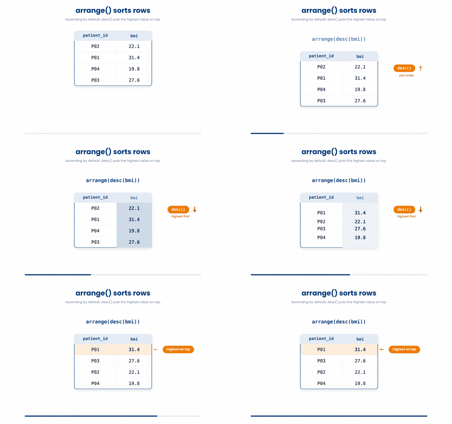
3.2 count(): tally how many fall in each group
count() tallies the rows. count(sex) returns one row per sex with a column n giving how many patients have each value. It is the fastest way to answer "how many in each group?".
Try this snippet in the R Scratchpad on the right.
library(dplyr)
library(readr)
patients <- read_csv("patients.csv")
patients |>
    count(smoker)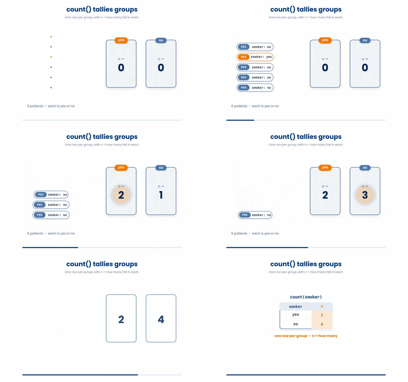
You can build a tiny tibble by hand to see exactly how a count works. Here are six recorded smoking statuses; counting how many are "yes" is just summing a logical test.
4 mutate() derives new clinical variables
Filtering, selecting, and sorting only ever show you data that is already there. mutate() is different: it adds a new column computed from existing ones, leaving every original column in place. This is how you derive the clinical variables your analysis actually needs.
mutate(bmi_rounded = round(bmi, 1)) adds a column called bmi_rounded. The name on the left is new; the expression on the right is computed for every row. You can derive several columns in one mutate() call, separated by commas.
Try this snippet in the R Scratchpad on the right.
library(dplyr)
library(readr)
patients <- read_csv("patients.csv")
patients |>
    mutate(bmi_rounded = round(bmi, 1))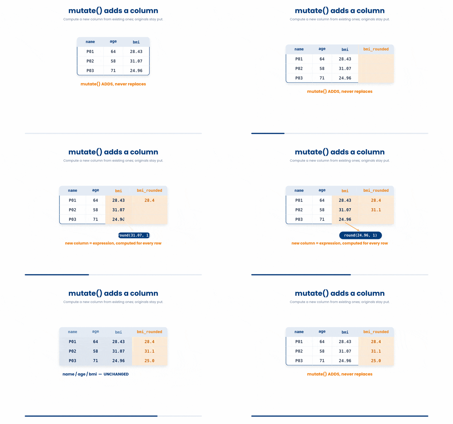
4.1 if_else(): one yes/no rule
For a single two-way rule, use if_else(). You give it a condition, the value to use when it is TRUE, and the value when it is FALSE. if_else(bmi >= 30, "obese", "not obese") labels each patient by one threshold.
Try this snippet in the R Scratchpad on the right.
library(dplyr)
library(readr)
patients <- read_csv("patients.csv")
patients |>
    mutate(obese = if_else(bmi >= 30, "obese", "not obese"))
4.2 case_when(): several rules at once
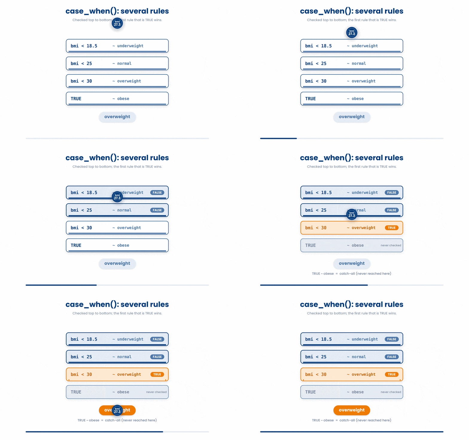
When you need more than two categories, reach for case_when(). You write each rule as condition ~ value, and R checks them top to bottom, using the first one that is TRUE. This is how you build a BMI category from the standard cut-points.
case_when() stops at the first matching rule, so order the rules from lowest cut-point upward and they will not overlap. End with TRUE ~ "..." as a catch-all for anything left over.
Try this snippet in the R Scratchpad on the right.
library(dplyr)
library(readr)
patients <- read_csv("patients.csv")
patients |>
    mutate(bmi_cat = case_when(
    bmi < 18.5 ~ "underweight",
    bmi < 25 ~ "normal",
    bmi < 30 ~ "overweight",
    TRUE ~ "obese"
  ))
Here is the trap that catches everyone once. A dplyr verb returns a NEW data frame and never changes the original. Running patients |> mutate(...) prints a changed table, but patients itself is untouched. To keep the result, assign it back with <-, or keep piping into the next step.
Now feel the payoff of the pipe: chain three verbs into one readable pipeline. Read it aloud as "take patients, THEN keep ages over 50, THEN keep three columns, THEN sort by BMI".
Try this snippet in the R Scratchpad on the right.
library(dplyr)
library(readr)
patients <- read_csv("patients.csv")
patients |>
  filter(age > 50) |>
  select(patient_id, age, bmi) |>
  arrange(desc(bmi))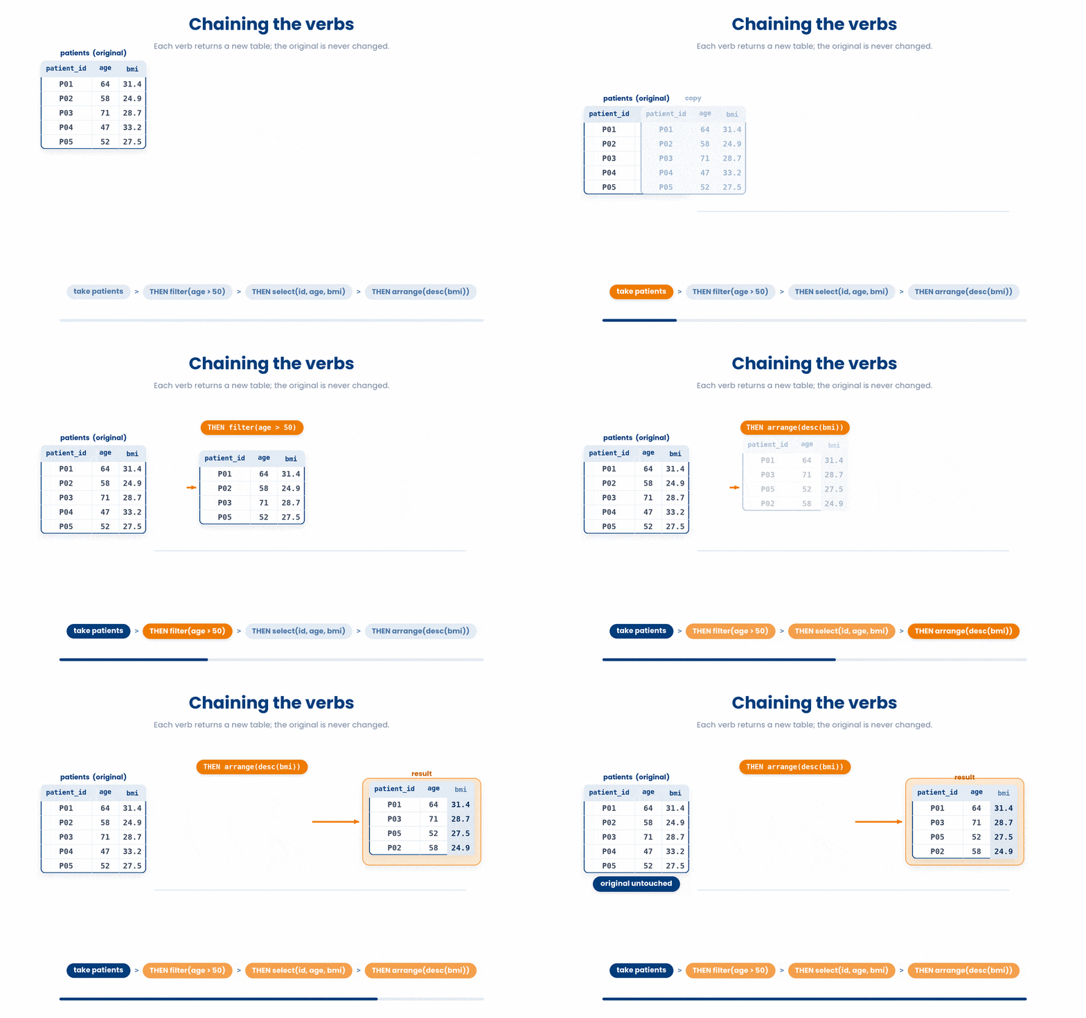
5 Put it together
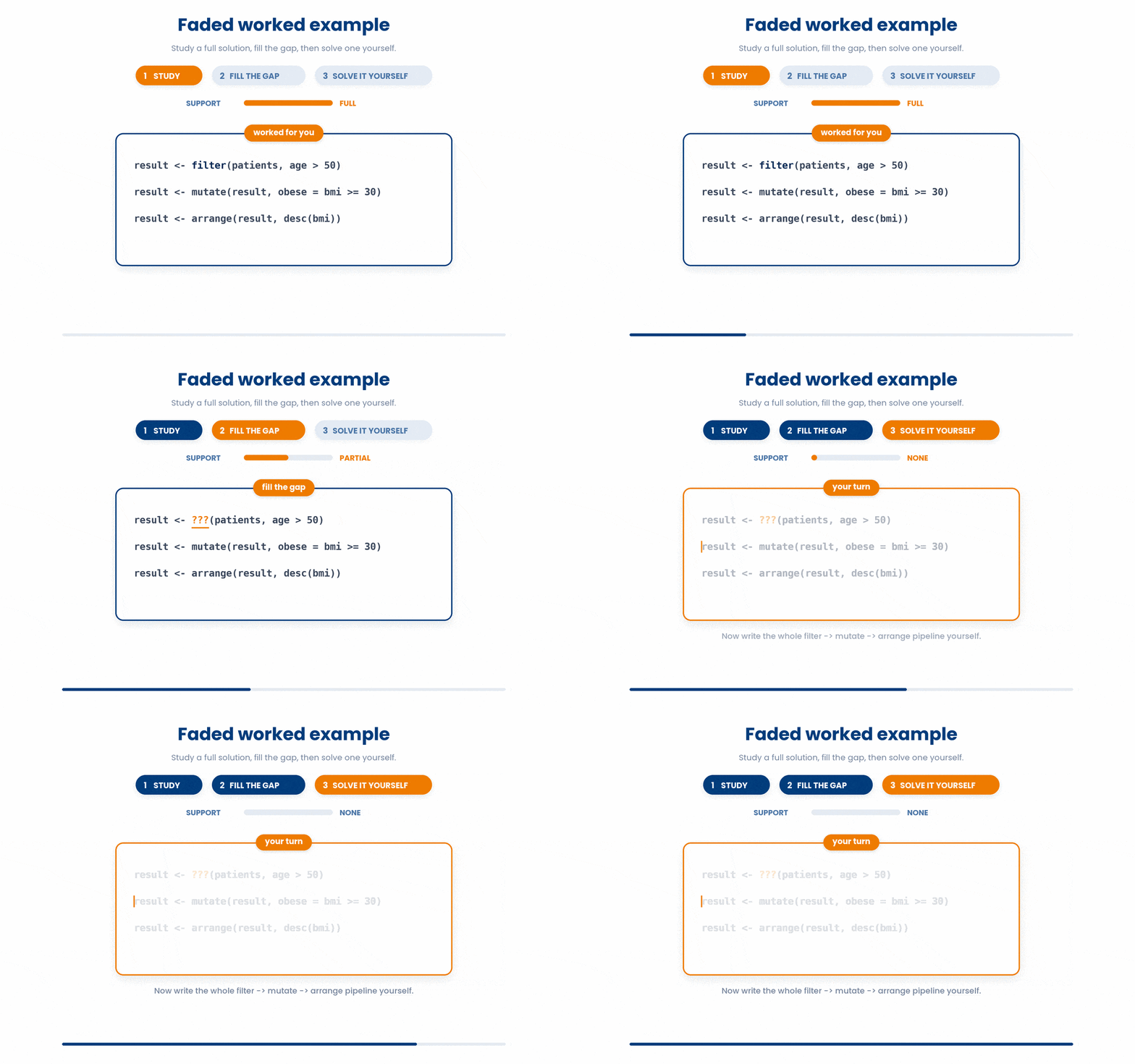
Now chain the verbs into one analysis. The worked example below writes each step as result <- verb(result, ...), which runs the verbs in order exactly as a |> pipeline would. It fades the support as you go: first you study a full solution, then you fill the gaps, then you solve a fresh one on your own.
Work through this example in three stages. You unlock each stage only after the tutor confirms the previous one. Each stage removes more of the scaffolding — by the end you are writing it yourself.
Problem: From patients.csv, keep only patients aged over 50, add a column flagging obesity (BMI of 30 or more), and sort the result so the highest BMI is on top.
library(dplyr)
library(readr)
patients <- read_csv("patients.csv")
result <- filter(patients, age > 50)
result <- mutate(result, obese = if_else(bmi >= 30, "obese", "not obese"))
result <- arrange(result, desc(bmi))
result- Read patients.csv into a tibble and switch on dplyr
- filter() keeps only the rows where age is over 50
- mutate() adds the obese flag with one if_else() rule
- arrange() with desc() sorts so the highest BMI is first
The same solution with key parts replaced by ???.
Fill in every ??? so the code matches the reference,
then ask the tutor to check it.
Your turn: Now do the same idea for a different group: keep only smokers, add a column high_bmi that is "high" when BMI is 25 or more and "ok" otherwise, and sort by age from youngest to oldest.
This Parsons problem gives you the right lines in the wrong order, plus a few lines that do not belong. Each line reassigns result, so the ordering is what matters: you must filter before you sort. Drag the correct lines into order and leave the wrong ones in the bank.
All the lines you need are in the Line bank on the left — some may be distractors you should leave behind. Drag the lines you need into the Your solution column on the right, in the correct order, then click Check.
Task: Switch on the packages and read patients.csv, then keep ages over 60, add a BMI category with case_when(), and sort by that category. Each step reassigns result.
result <- filter(patients, age > 60)result <- select(patients, age > 60)result <- mutate(result, bmi_cat = case_when(bmi < 25 ~ "normal", bmi < 30 ~ "overweight", TRUE ~ "obese"))library(dplyr)library(readr)result <- arrange(result, bmi_cat)patients <- read_csv("patients.csv")result <- filter(patients) > 60result <- mutate(result, bmi_cat = if_else(bmi < 25, bmi < 30, "obese"))
- Drop lines here, in order.
6 Check your understanding
You have reached the end of the module. Try the same questions again — your answers here, paired with your pre-test answers, are how we measure what the module taught you. Answer every question and confidence rating, then click Submit and see results to view your score.
Which line sorts patients so the highest BMI is on top?
By default, arrange(age) orders the rows how?
Which line tells you how many patients fall into each smoking-status group?
In the tibble returned by count(sex), what does the column n contain?
Which verb adds a new column while leaving every existing column in place?
You pipe patients into mutate() to add an obese column but do not assign the result. What happens to the patients tibble?
Which verb and helper would you use to label patients as "underweight", "normal", "overweight", or "obese" by BMI?
In case_when(), when several rules could match a row, which rule's value is used?
I can use arrange() with desc() to sort a table in either direction, and count() to tally how many patients fall in each group.
I can use mutate() to add a new clinical variable computed from existing columns, and explain that a dplyr verb returns a new data frame rather than changing the original.
I can use if_else() for a single two-way rule and case_when() for several ranked rules to label patients, and assign the result back with <- to keep it.
7 Your results
Here is how your post-test answers compare with your pre-test answers. The pre/post pairing is the most reliable way to see what this module actually taught you.
Submit the post-test to see your results.
What is the one thing from this module that is still unclear to you?