

1 Before you start
This is not graded, and it does not count towards anything. Answer every question even if you are only guessing — having a go at something before you have been taught it is one of the best ways to remember it afterwards. The lesson ends with another short check, and there you will be shown the correct answer for anything you missed. Choose an option for every question and confidence rating, then click Submit answers.
What does a dplyr verb such as filter() give you back?
Why can you chain dplyr verbs one after another?
How should you read the native pipe |> when you say a pipeline aloud?
The line patients |> filter(age > 60) is exactly the same call as which of the following?
Which verb keeps only the ROWS of a tibble that meet a condition, such as age over 60?
Which verb keeps only the COLUMNS patient_id, age, and bmi and drops the rest?
You want the patients who are over 60 AND are smokers. Which filter() call is correct?
Why does filter(patients, smoker = "yes") throw an error?
I can explain that every dplyr verb takes a data frame and returns one, which is why the verbs can be chained together.
I can read and write a |> pipeline aloud as "take the data, THEN ...", and know it is the same as passing the data as the first argument.
I can use filter() to keep the rows that meet a condition and select() to keep the columns I name, using == (not =) for equality.
2 Introduction
In Module 1 you loaded a clinical dataset into R and confirmed it came in correctly. Now you start to reshape it. Real data almost never arrives in the shape your analysis needs: you may want one age group, or just a handful of columns. This part gives you the shared rule behind every reshaping tool, the pipe that strings those tools together, and the first two verbs you will reach for.
This part of the module covers three foundations you will use in almost every analysis:
- One grammar — every dplyr verb takes a data frame as its first argument and returns a new data frame, so verbs chain together.
- The native pipe — read a pipeline aloud as "take the data, THEN do this, THEN do that".
- filter() and select() — keep the rows you want and the columns you need.
By the end of this part you will be able to explain why any dplyr verb can feed straight into the next, read and write a |> pipeline aloud as a sequence of steps, and keep exactly the rows and columns you want from a clinical table.
Try every snippet in the R Scratchpad on the right — the dataset patients.csv is already loaded and waiting for you.
3 One grammar: every verb takes a data frame and returns one
Everything in this part comes from one package, dplyr, which gives you a small set of verbs — functions named after the action they do, like filter, select, and mutate. dplyr is part of the tidyverse, the family of packages this course uses throughout.
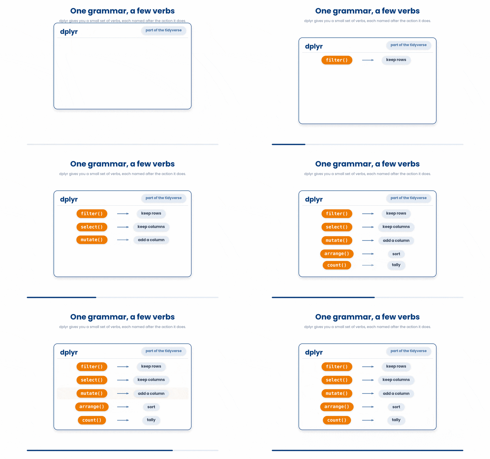
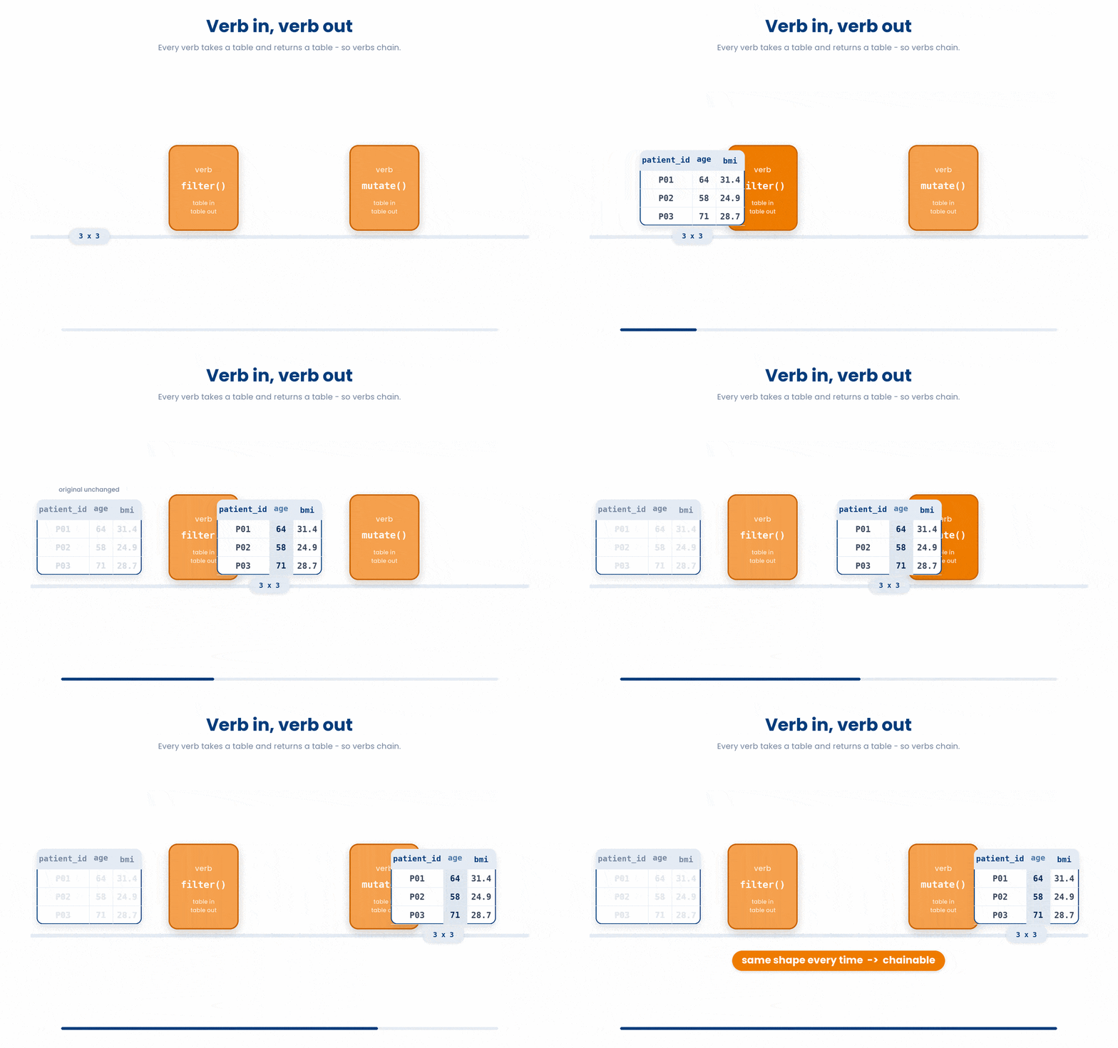
The verbs share one rule, and that rule is the whole trick. Every dplyr verb takes a data frame as its first argument and returns a new data frame. The output of one verb is therefore a valid input to the next, so you can chain them into a pipeline that reads like a recipe.
A data frame is just a table: one row per patient, one column per variable. The tidyverse's tidy version of a table is a tibble, which is what read_csv() handed you in Module 1. Verb in, verb out — same shape of object every time.
First, switch the package on for the session with library(). You call library(dplyr) once at the top of your script, not before every line.
Try this snippet in the R Scratchpad on the right.
library(dplyr)
library(readr)
patients <- read_csv("patients.csv")
patients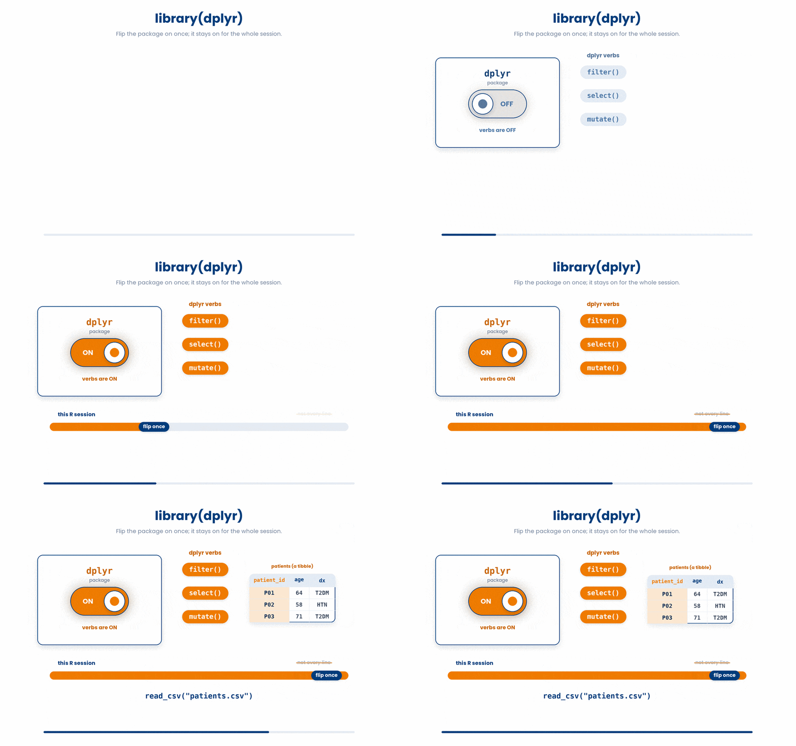
4 The native pipe |>: reading a pipeline aloud
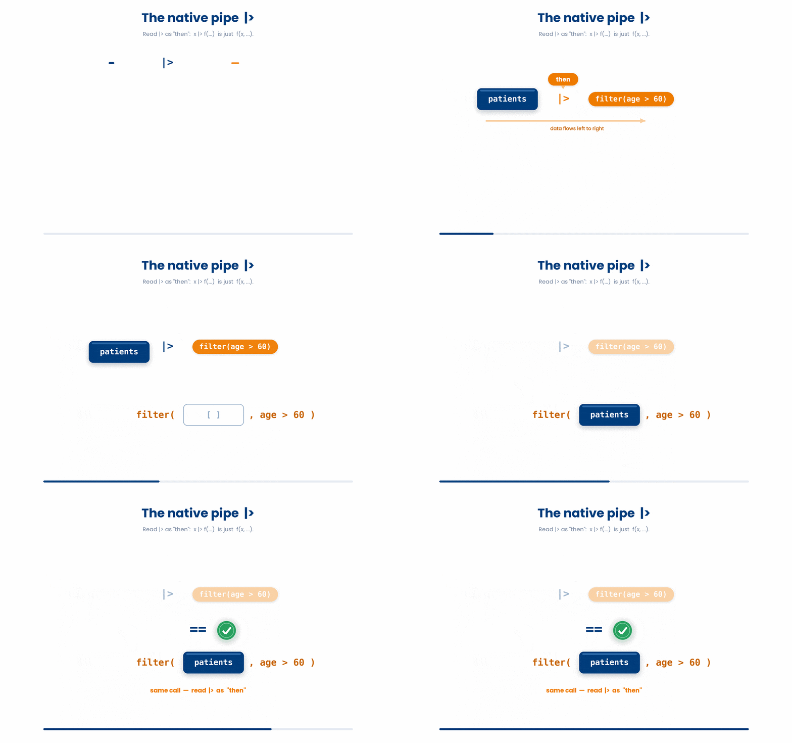
Because every verb returns a data frame, you could nest them — but that reads inside-out and quickly becomes unreadable. Instead you use the native pipe, written |>, which takes the result on its left and feeds it as the first argument to the function on its right.
Read |> aloud as the word then. The line patients |> filter(age > 60) says "take patients, THEN filter to ages over 60". The data flows left to right, top to bottom, in the same order you would say the steps out loud.
Writing each step on its own line makes a pipeline read like a numbered procedure. The pipe at the end of a line tells R the pipeline continues onto the next line.
Because the pipe just supplies the data frame as the first argument, patients |> filter(age > 60) does exactly the same thing as writing the data frame inside the verb: filter(patients, age > 60). The pipeline form is easier to read once you chain several steps, so prefer it — but the two are interchangeable, and you will see both.
Try this snippet in the R Scratchpad on the right.
library(dplyr)
library(readr)
patients <- read_csv("patients.csv")
patients |>
    filter(age > 60)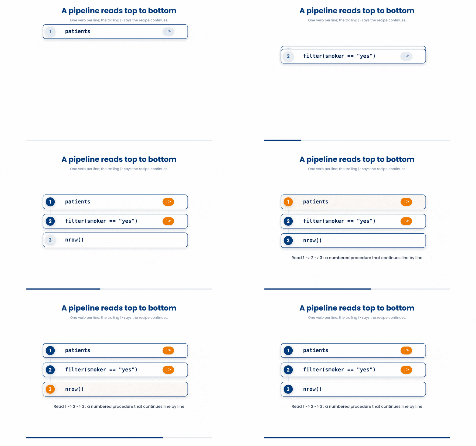
5 filter() keeps rows while select() keeps columns
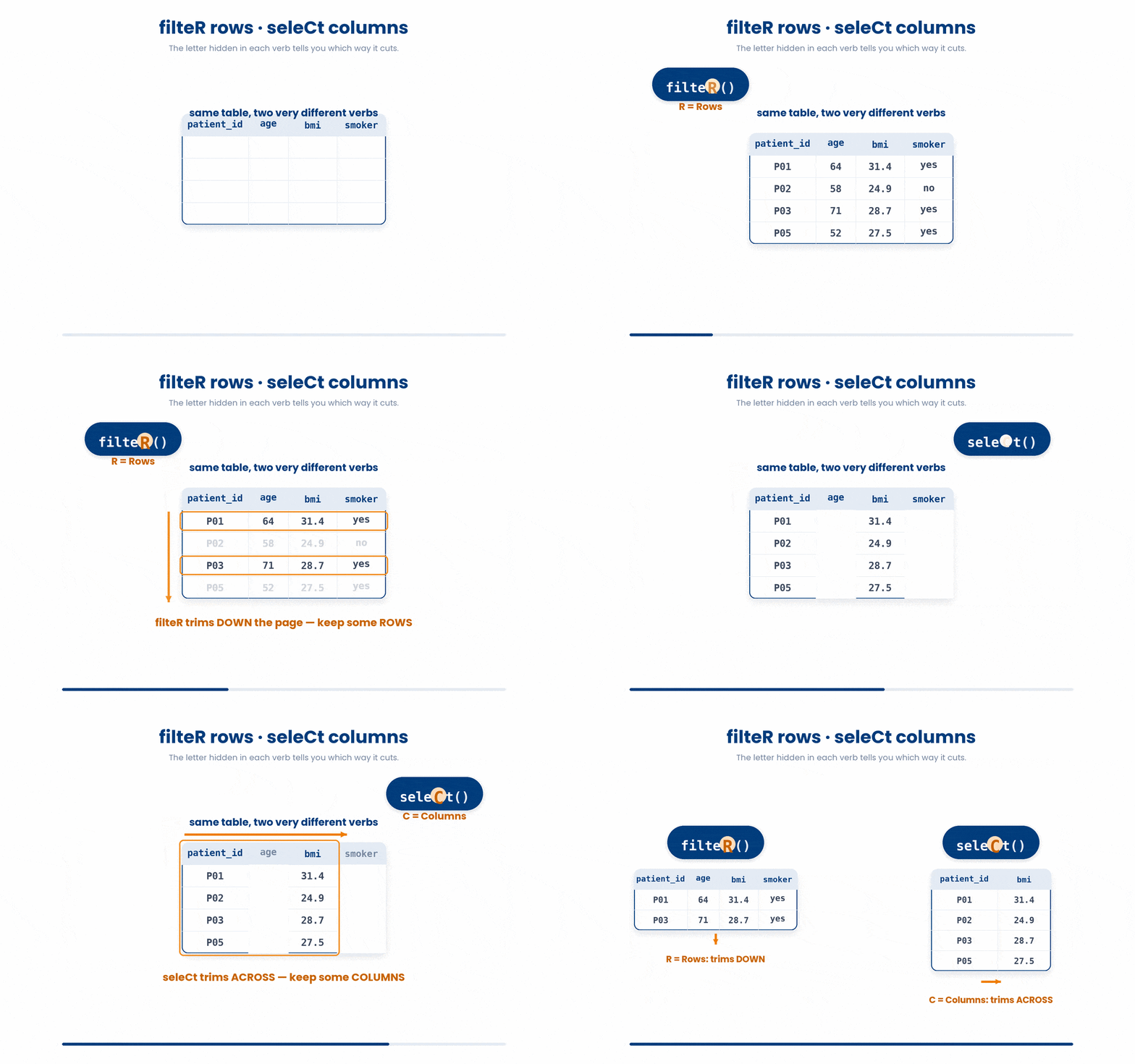
The filter() and select() are two verbs you will use most often do opposite jobs. One trims the table down the page; the other trims it across. Keeping them straight is the single most useful habit in this part.
5.1 filter(): keep the ROWS that match a condition
filter() keeps the rows where a condition is TRUE and drops the rest. You give it a test such as age > 60 or smoker == "yes". Note the double equals == for "is equal to" — a single = means assignment, not a comparison.
Combine conditions with & for "and" and | for "or". filter(age > 60 & smoker == "yes") keeps patients who are both over 60 and smokers.
Try this snippet in the R Scratchpad on the right.
library(dplyr)
library(readr)
patients <- read_csv("patients.csv")
patients |>
    filter(age > 60, smoker == "yes")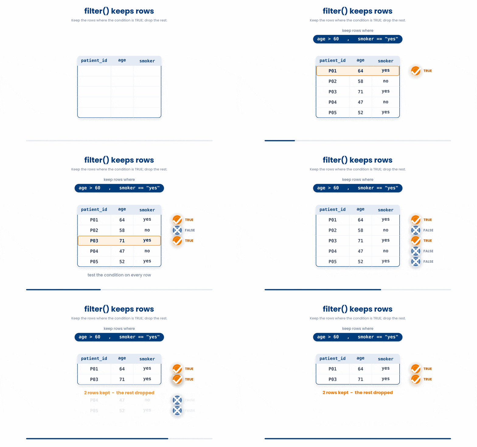
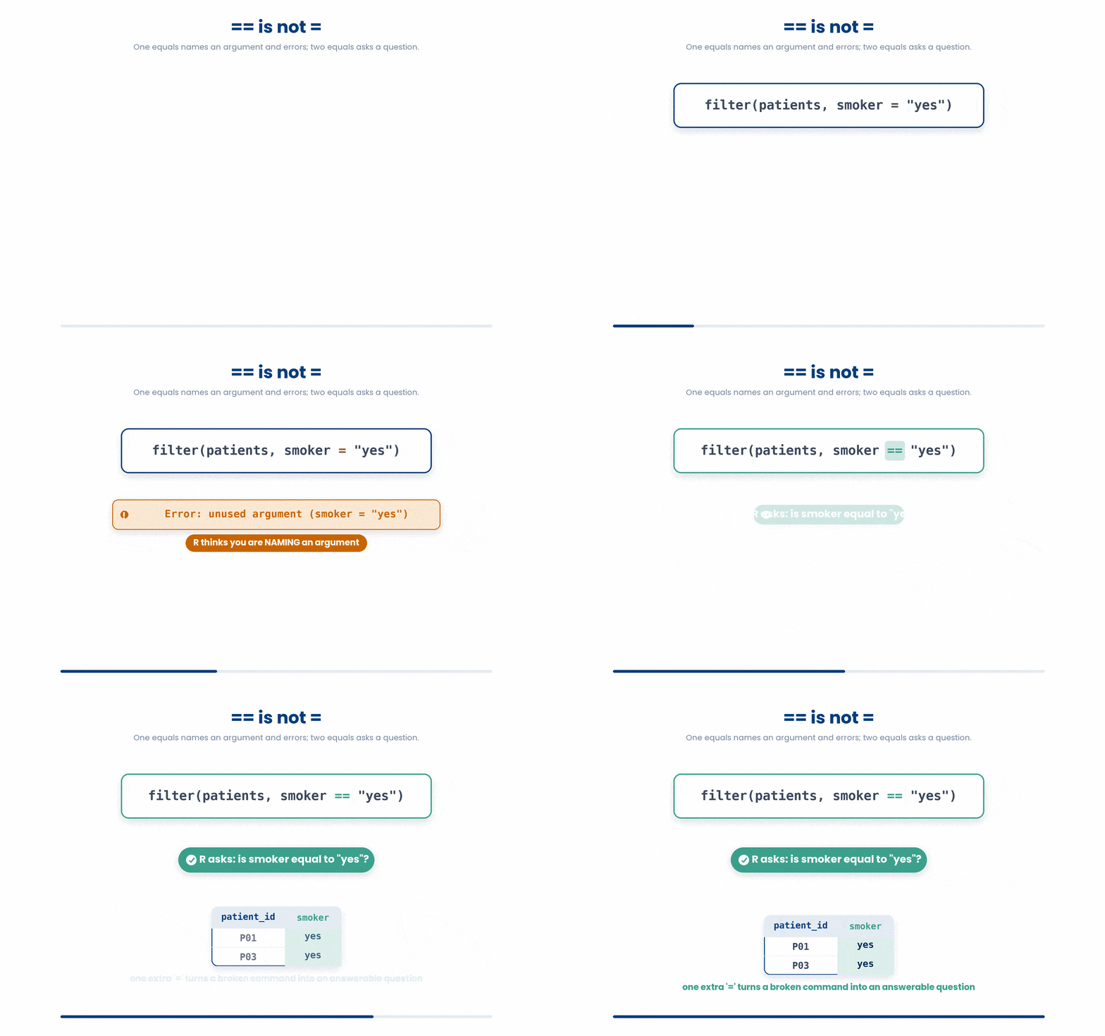
Watch the ==. Writing filter(smoker = "yes") with one equals is a classic trap — R reads it as trying to set an argument named smoker and throws an error. Use == whenever you mean "is equal to".
The code below is broken. Type a fixed version into the editor, then click Run & check. Success means your code runs without errors. Use Show hint only if you get stuck.
library(dplyr)
library(readr)
patients <- read_csv("patients.csv")
filter(patients, smoker = "yes")- Use == to test equality: filter(patients, smoker == "yes") ★
- Wrap the value in c(): filter(patients, smoker == c("yes"))
- Drop the quotes: filter(patients, smoker == yes)
5.2 select(): keep the columns you name
select() keeps only the columns you list by name and drops the rest. select(patient_id, age, bmi) returns a narrower table with just those three columns, in the order you wrote them.
Try this snippet in the R Scratchpad on the right.
library(dplyr)
library(readr)
patients <- read_csv("patients.csv")
patients |>
    select(patient_id, age, bmi)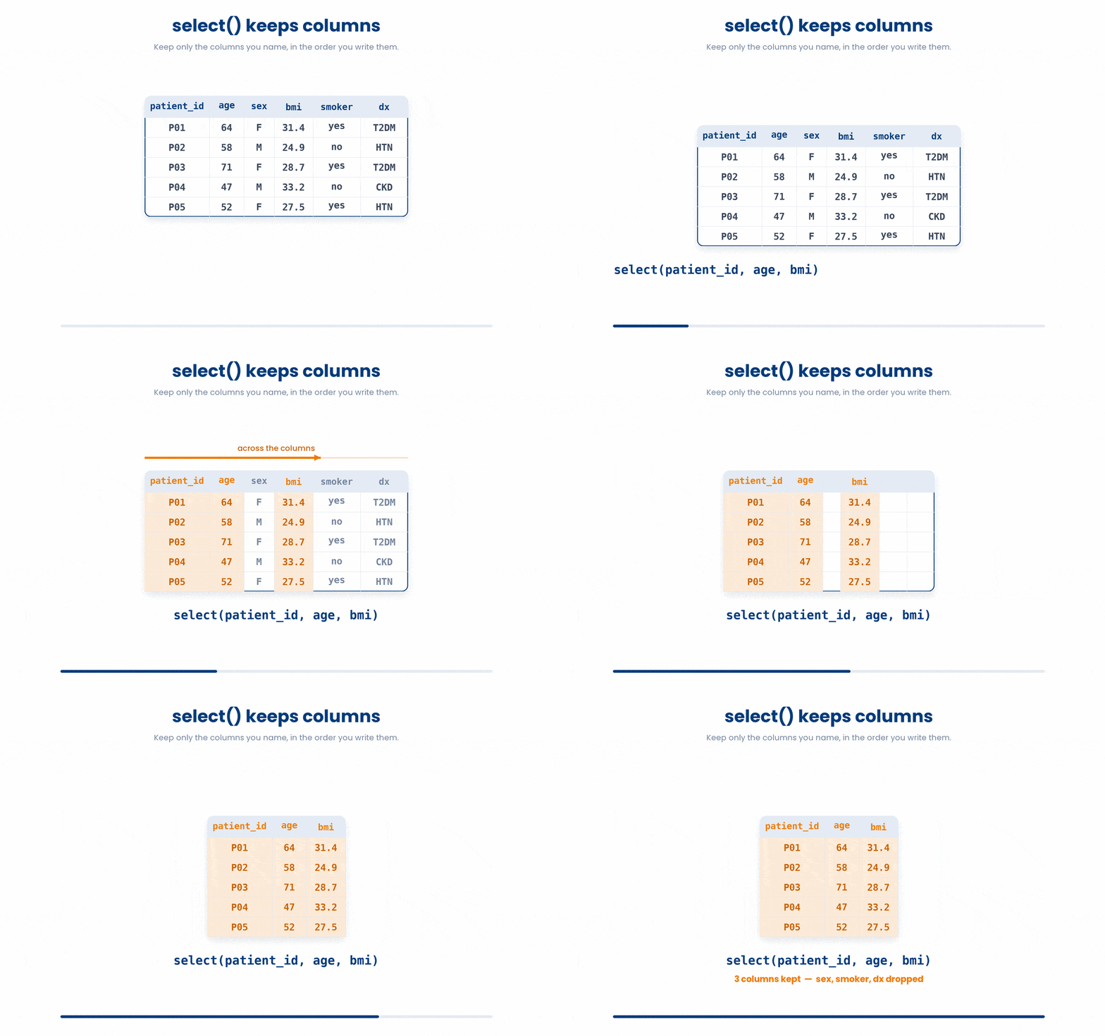
The classic mix-up is using filter() when you meant select(), or the reverse. A mnemonic fixes it: filteR ends in R for Rows; seleCt has a C for Columns.
Let’s try and practise by trimming the table down the page and across in one pipeline.
Work through this example in three stages. You unlock each stage only after the tutor confirms the previous one. Each stage removes more of the scaffolding — by the end you are writing it yourself.
Problem: From patients, keep patients older than 50, then keep only their patient_id and diagnosis columns.
library(dplyr)
library(readr)
patients <- read_csv("patients.csv")
patients |>
    filter(age > 50) |>
select(patient_id, diagnosis)- filter() keeps the rows where age exceeds 50
- select() then keeps only the two named columns
- the pipe feeds the filtered table straight into select()
The same solution with key parts replaced by ???.
Fill in every ??? so the code matches the reference,
then ask the tutor to check it.
Your turn: Keep only patients older than 60, select their patient_id and bmi, and report how many rows remain with nrow().
6 Check your understanding
You have reached the end of the module. Try the same questions again — your answers here, paired with your pre-test answers, are how we measure what the module taught you. Answer every question and confidence rating, then click Submit and see results to view your score.
What does a dplyr verb such as filter() give you back?
Why can you chain dplyr verbs one after another?
How should you read the native pipe |> when you say a pipeline aloud?
The line patients |> filter(age > 60) is exactly the same call as which of the following?
Which verb keeps only the ROWS of a tibble that meet a condition, such as age over 60?
Which verb keeps only the COLUMNS patient_id, age, and bmi and drops the rest?
You want the patients who are over 60 AND are smokers. Which filter() call is correct?
Why does filter(patients, smoker = "yes") throw an error?
I can explain that every dplyr verb takes a data frame and returns one, which is why the verbs can be chained together.
I can read and write a |> pipeline aloud as "take the data, THEN ...", and know it is the same as passing the data as the first argument.
I can use filter() to keep the rows that meet a condition and select() to keep the columns I name, using == (not =) for equality.
7 Your results
Here is how your post-test answers compare with your pre-test answers. The pre/post pairing is the most reliable way to see what this module actually taught you.
Submit the post-test to see your results.
What is the one thing from this module that is still unclear to you?