

1 Before you start
This is not graded, and it does not count towards anything. Answer every question even if you are only guessing — having a go at something before you have been taught it is one of the best ways to remember it afterwards. The lesson ends with another short check, and there you will be shown the correct answer for anything you missed. Choose an option for every question and confidence rating, then click Submit answers.
The file diabetes_clinic.csv is in your workspace. Which line reads it into R and stores it in an object called clinic?
read_csv() lives in the readr package. Which line switches that package on for the session before you use it?
read_csv() returns a tibble. What does the tibble printout tell you under each column name that helps you check the load?
You have just run clinic <- read_csv("diabetes_clinic.csv"). Which line lists every column down the page with its type and first values, to confirm it loaded correctly?
A tibble called clinic has a column age. Which line pulls that column out as a vector so you can run mean() on it?
You want the average HbA1c across the loaded clinic dataset. Which line does this?
What makes a Quarto (.qmd) report reproducible?
Your data is in an Excel worksheet rather than a .csv. Which function reads it into a tibble?
I can read a .csv into R with read_csv() from readr, after switching the package on with library(), and store the result in a named object.
I can confirm a dataset loaded correctly using the tibble printout, glimpse(), and head(), and pull out a single column as a vector with $.
I can explain what a Quarto (.qmd) report is and why rendering it from the raw data and code makes an analysis reproducible.
2 Introduction
In Part I you built values and vectors by hand with <- and c(). Real clinical data does not arrive one value at a time — it lives in a file. This part takes you from a file on disk to a loaded, checked dataset, and then to a report that computes every number in it from that raw data instead of copying it by hand.
This part of the module covers three foundations you will reach for in every analysis that follows:
- Reading data — loading a .csv file into R with read_csv() and giving the result a name you can work with.
- Checking the load — using the tibble printout, glimpse(), and head() to confirm every column came in as the type you expected.
- Reproducible reports — writing a Quarto document that mixes your prose with runnable code, so one render rebuilds the whole report from the data.
By the end of this part you will be able to read a clinical dataset into R with read_csv(), confirm it loaded correctly with glimpse() and head(), pull a single column out as a vector with $, and explain why a Quarto report is reproducible when a copy-and-pasted number is not.
Try every snippet in the R Scratchpad on the right — the dataset diabetes_clinic.csv is already loaded and waiting for you.
3 Reading clinical data into R
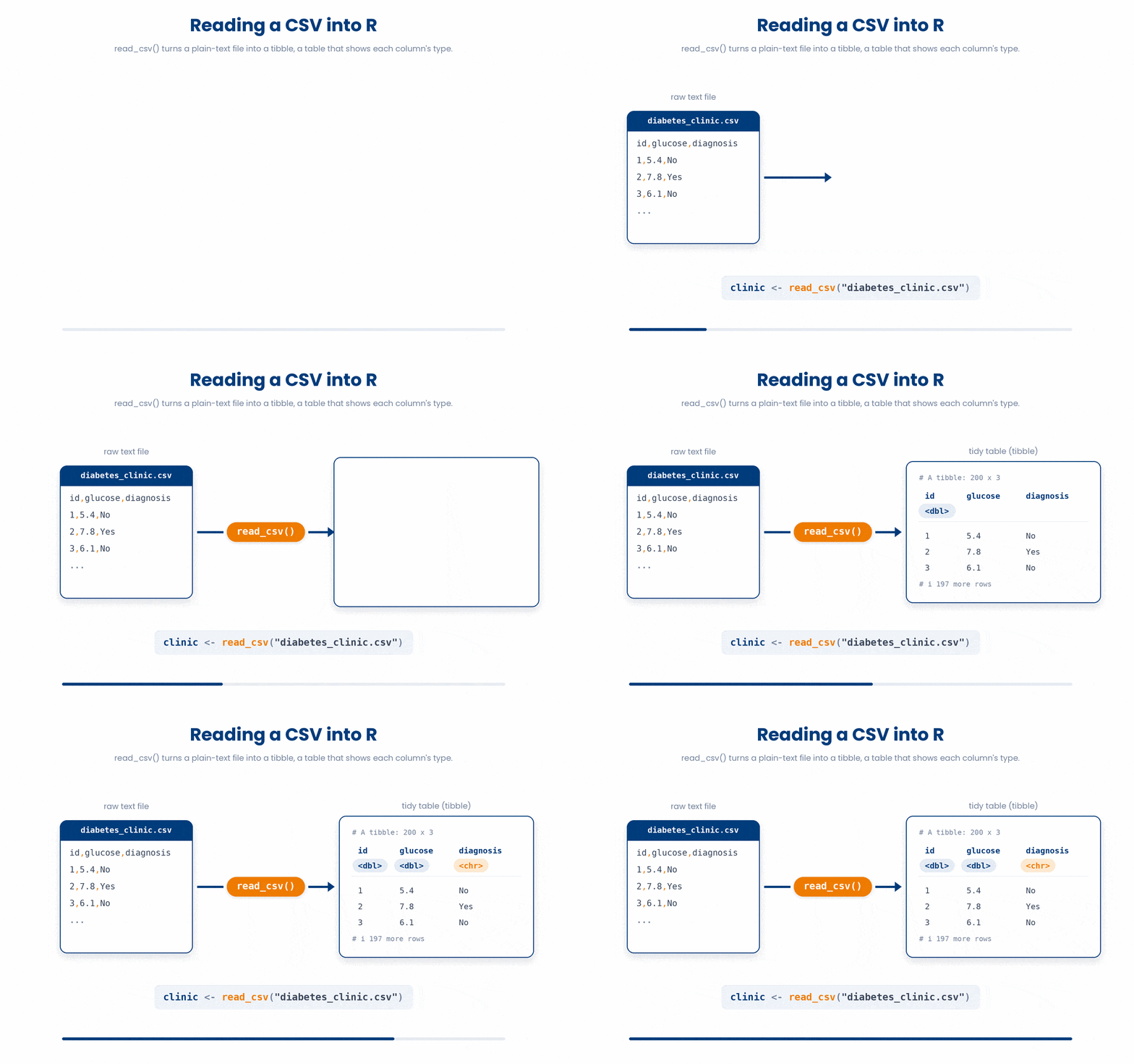
Clinical data usually lives in a .csv file — a plain-text table with one row per patient. You read one into R with read_csv() from the readr package.
A package is a bundle of extra functions; you switch it on for the session with library(). readr is part of the tidyverse, the family of packages this course uses throughout.
The file diabetes_clinic.csv is already in your workspace. Read it in and give it a name:
Try this snippet in the R Scratchpad on the right.
library(readr)
clinic <- read_csv("diabetes_clinic.csv")
clinicWhat you get back is a tibble — the tidyverse's tidy version of a table. A tibble prints cleanly: it shows the first ten rows, and under each column name it tells you the column's type (dbl for a number, chr for text, and so on), so you can spot at a glance whether a column came in as you expected.
Two functions help you confirm the data loaded correctly. glimpse() lists every column down the page with its type and first few values; head() shows the first six rows across.
Try this snippet in the R Scratchpad on the right.
library(readr)
library(dplyr)
clinic <- read_csv("diabetes_clinic.csv")
glimpse(clinic)
head(clinic)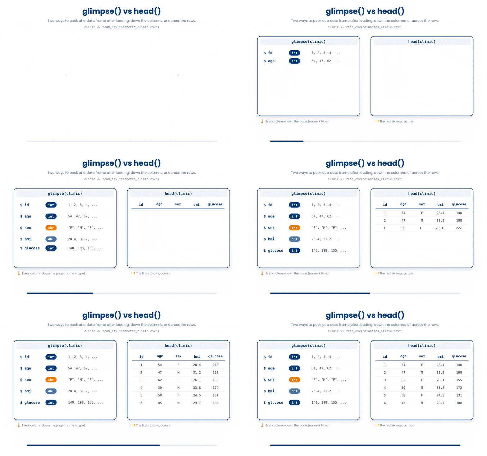
To pull one column out as a vector, write the dataset name, a dollar sign, and the column name: clinic$age is every patient's age.
Try this snippet in the R Scratchpad on the right.
library(readr)
clinic <- read_csv("diabetes_clinic.csv")
clinic$age
mean(clinic$age)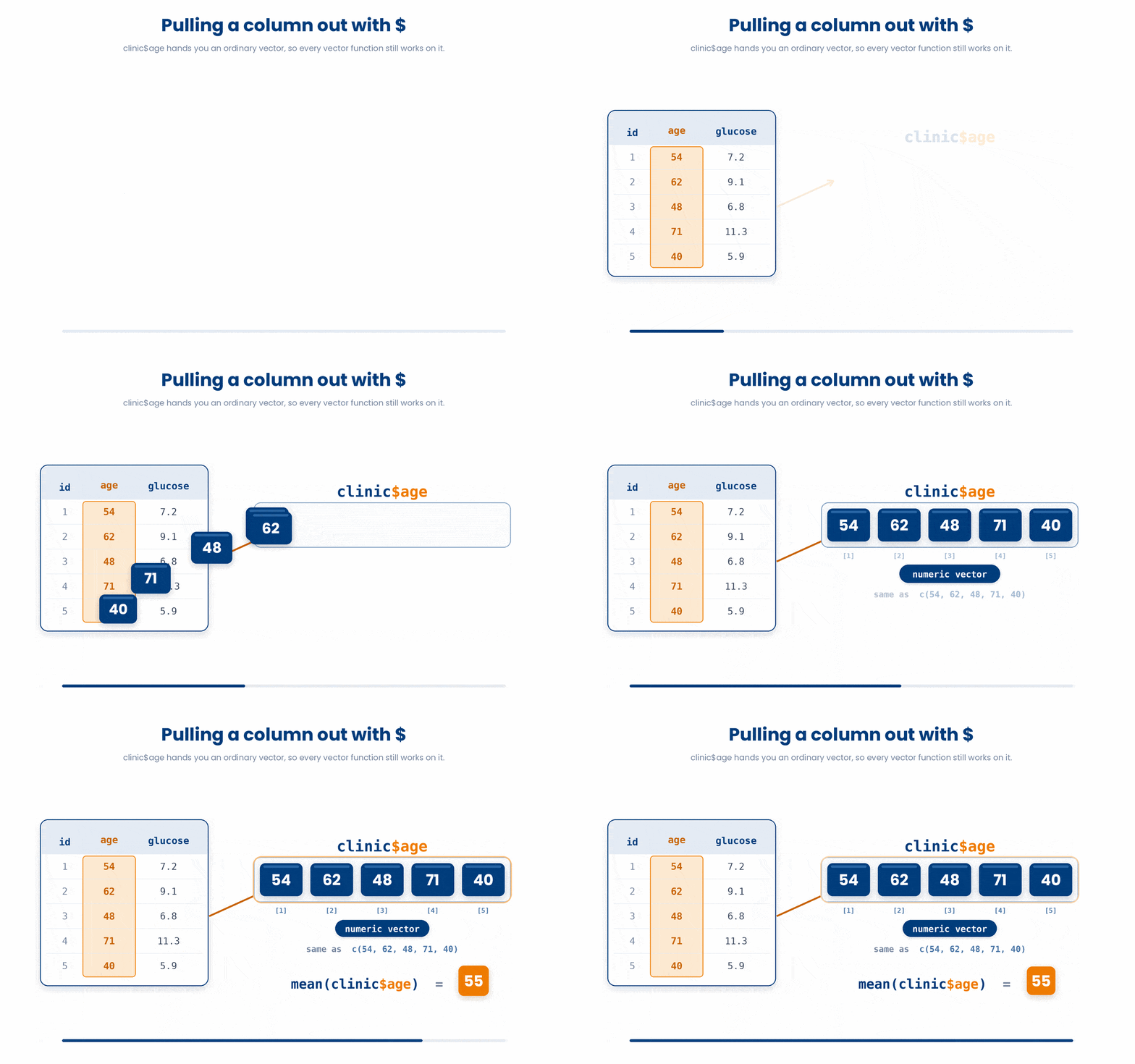
Excel files work almost the same way: read_excel("file.xlsx") from the readxl package reads a worksheet into a tibble. Reach for read_csv() when you can, though — a plain .csv is readable on any machine and never hides formatting surprises.
4 Reproducible reports with Quarto
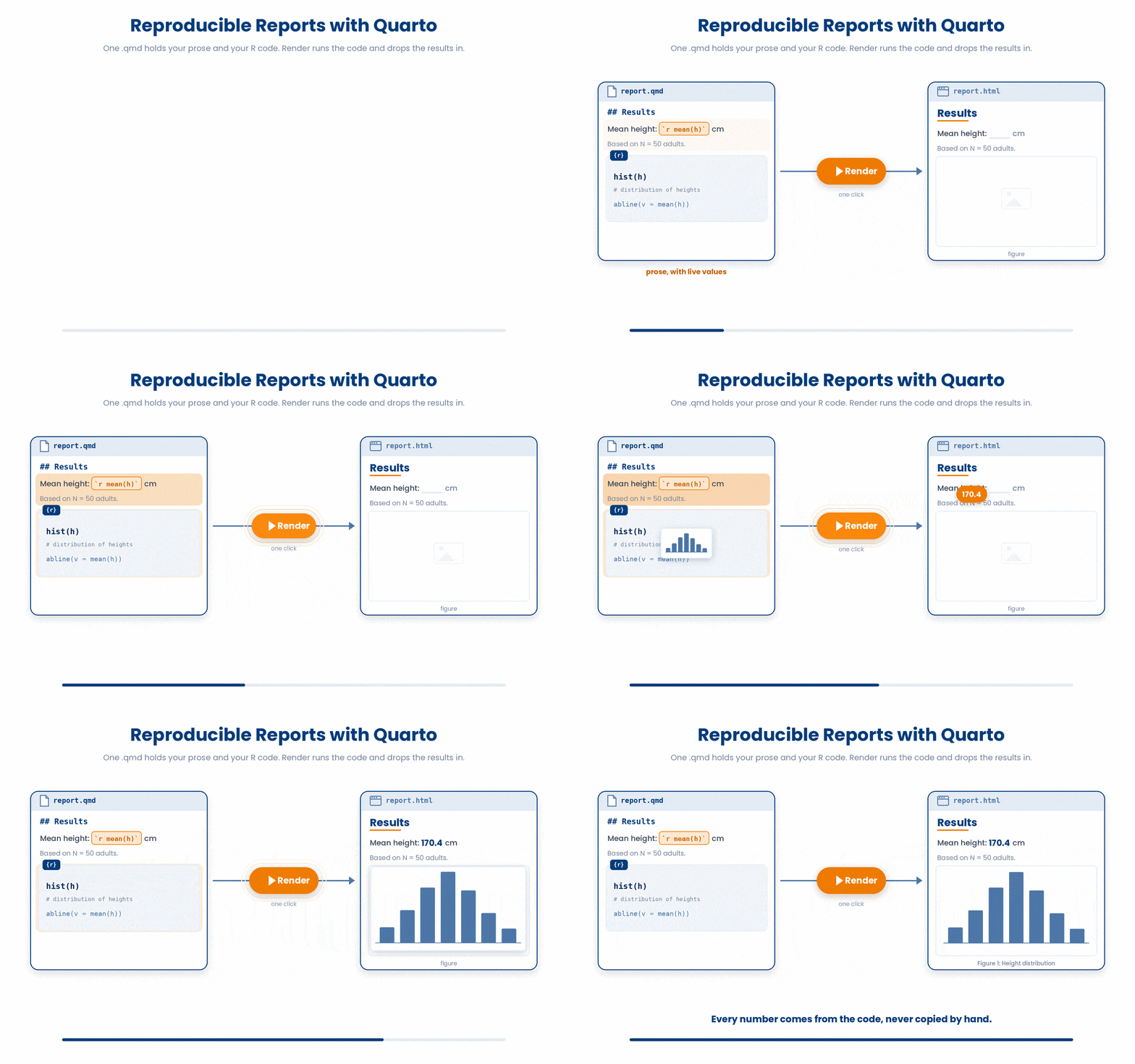
There is one more piece you will use: Quarto. A Quarto document (a .qmd file) mixes your written explanation with runnable R code in the same file. When you render it, R runs every code chunk fresh and drops the results — numbers, tables, plots — straight into a finished HTML, PDF, or Word report.
This matters because it makes your analysis reproducible: the report is generated from the raw data and the code in one click, so no number is ever copied by hand. You will write Quarto reports in RStudio for your labs; the in-browser scratchpad here is just for trying things out.
5 Put it together
Before you start on a worked example, let’s try and familiarize yourself with the syntax first.
This Parsons problem gives you the right lines in the wrong order, plus a few lines that do not belong. Drag the correct lines into order and leave the wrong ones in the bank.
All the lines you need are in the Line bank on the left — some may be distractors you should leave behind. Drag the lines you need into the Your solution column on the right, in the correct order, then click Check.
Task: Switch on readr, read the clinic file into an object called clinic, then show its first rows.
clinic <- read_csv("diabetes_clinic.csv")library(readr)head[clinic]head(clinic)library(read_csv)clinic <- read.csv(diabetes_clinic.csv)
- Drop lines here, in order.
The worked example below fades the support as you go: first you study a full solution, then you fill the gaps, then you solve a fresh one on your own.
Work through this example in three stages. You unlock each stage only after the tutor confirms the previous one. Each stage removes more of the scaffolding — by the end you are writing it yourself.
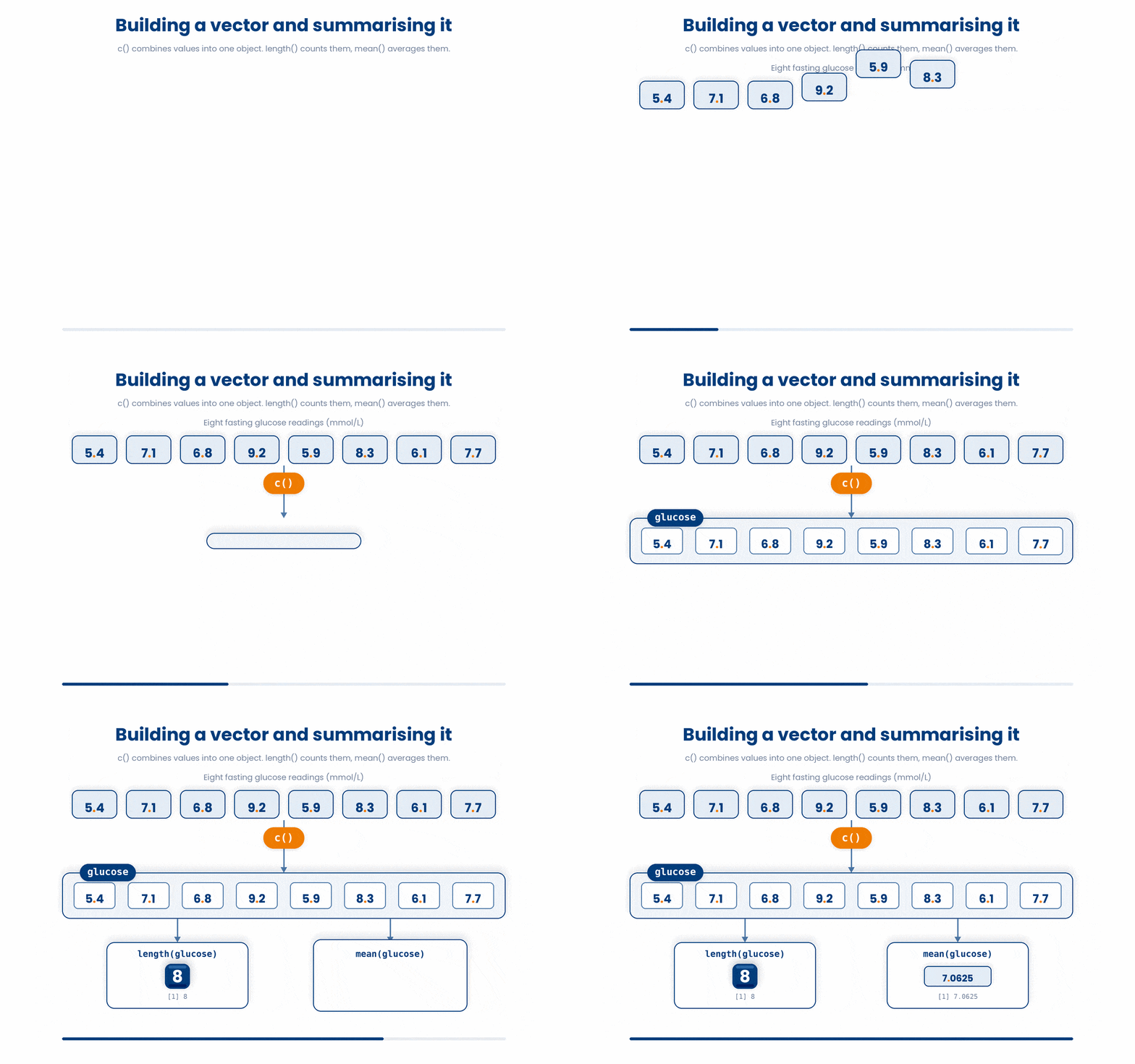
Problem: You have eight fasting glucose readings (mmol/L). Store them in one object, then report how many there are and their average.
glucose <- c(5.4, 7.1, 6.8, 9.2, 5.9, 8.3, 6.1, 7.7)
length(glucose)
mean(glucose)- Combine the eight readings into one vector with c()
- length() counts how many values the vector holds
- mean() adds them up and divides by the count
The same solution with key parts replaced by ???.
Fill in every ??? so the code matches the reference,
then ask the tutor to check it.
Your turn: Now do the same for four HbA1c results: 7.2, 8.1, 6.5, 9.4. Store them in an object called hba1c and report the average.
6 Check your understanding
You have reached the end of the module. Try the same questions again — your answers here, paired with your pre-test answers, are how we measure what the module taught you. Answer every question and confidence rating, then click Submit and see results to view your score.
The file diabetes_clinic.csv is in your workspace. Which line reads it into R and stores it in an object called clinic?
read_csv() lives in the readr package. Which line switches that package on for the session before you use it?
read_csv() returns a tibble. What does the tibble printout tell you under each column name that helps you check the load?
You have just run clinic <- read_csv("diabetes_clinic.csv"). Which line lists every column down the page with its type and first values, to confirm it loaded correctly?
A tibble called clinic has a column age. Which line pulls that column out as a vector so you can run mean() on it?
You want the average HbA1c across the loaded clinic dataset. Which line does this?
What makes a Quarto (.qmd) report reproducible?
Your data is in an Excel worksheet rather than a .csv. Which function reads it into a tibble?
I can read a .csv into R with read_csv() from readr, after switching the package on with library(), and store the result in a named object.
I can confirm a dataset loaded correctly using the tibble printout, glimpse(), and head(), and pull out a single column as a vector with $.
I can explain what a Quarto (.qmd) report is and why rendering it from the raw data and code makes an analysis reproducible.
7 Your results
Here is how your post-test answers compare with your pre-test answers. The pre/post pairing is the most reliable way to see what this module actually taught you.
Submit the post-test to see your results.
What is the one thing from this module that is still unclear to you?