

1 Before you start
This is not graded, and it does not count towards anything. Answer every question even if you are only guessing — having a go at something before you have been taught it is one of the best ways to remember it afterwards. The lesson ends with another short check, and there you will be shown the correct answer for anything you missed. Choose an option for every question and confidence rating, then click Submit answers.
You have a fitted logistic model fit and want each patient's estimated probability of the event. Which call returns probabilities rather than log-odds?
You run predict(fit) on a logistic model without setting type. What scale are the returned values on?
A colleague reports that their prediction model has an AUC of 0.50. How should you read that?
Which pair of calls measures a logistic model's discrimination, given the true 0/1 outcome and the predicted probabilities?
A patient reaches the end of the study still alive, so their time to death is unknown. In survival analysis this observation is described as
The lung dataset codes its status column as 1 = censored and 2 = dead. Before building a Surv() outcome, why must you recode it so 1 = event?
Which function estimates the Kaplan-Meier survival curve, split by treatment group?
A log-rank test comparing survival in two arms returns p = 0.002. What may you conclude?
I can generate predicted probabilities from a logistic model with predict(type = "response") and explain why the default returns log-odds instead.
I can measure a model's discrimination by building an ROC curve with roc() and reading its AUC, and I know that 0.5 is a coin flip and 1.0 is perfect.
I can code a censored time-to-event outcome with Surv(time, event), draw a Kaplan-Meier curve, and compare two groups with the log-rank test via survdiff() while knowing its limits.
2 Introduction
In Part III you fit a logistic model and turned its coefficients into adjusted odds ratios. A fitted model can do more than report effects — it can predict. This part asks each patient's estimated risk, checks how well those risks separate patients who had the event from those who did not, and then steps into a different kind of question altogether: not whether an event happens, but when.
This part of the module covers two skills:
- Predicted probabilities and discrimination — read each patient's estimated risk with predict() and type = "response", then measure how well those risks separate the groups with an ROC curve and its AUC.
- A taste of survival analysis — handle censoring, pack time and status into an outcome with Surv(), draw a Kaplan-Meier curve, and compare two groups with the log-rank test.
By the end of this part you will be able to generate predicted probabilities from a logistic model, quantify its discrimination with an ROC AUC and read that number correctly, code a censored time-to-event outcome with Surv(), produce and interpret a Kaplan-Meier survival curve, and compare two groups with a log-rank test — while knowing exactly what that test can and cannot tell you.
Try every snippet in the R Scratchpad on the right. The discrimination examples build a small simulated cohort with set.seed() and score it with pROC; the survival examples use the lung dataset that ships inside the survival package.
3 Predicted probabilities and discrimination
A fitted model can also predict. Feed it the patients and ask for each one's estimated probability of the event with predict() and type = "response". The type = "response" part is essential: without it predict() returns log-odds, not probabilities.
Try this snippet in the R Scratchpad on the right.
set.seed(2025)
n <- 300
age <- round(rnorm(n, mean = 60, sd = 10))
smoker <- rbinom(n, 1, 0.35)
complication <- rbinom(n, 1, 1 / (1 + exp(-(-6 + 0.07 * age + 0.8 * smoker))))
cohort <- data.frame(age, smoker, complication)
fit <- glm(complication ~ age + smoker, family = binomial, data = cohort)
cohort$prob <- predict(fit, type = "response")
summary(cohort$prob)![On a fitted logistic model predict() returns log-odds by default (here -1.0), and type = "response" passes that value through the logistic curve to give the patient's event probability in [0, 1] (here 0.27).](GIF_predict_type_response.gif)
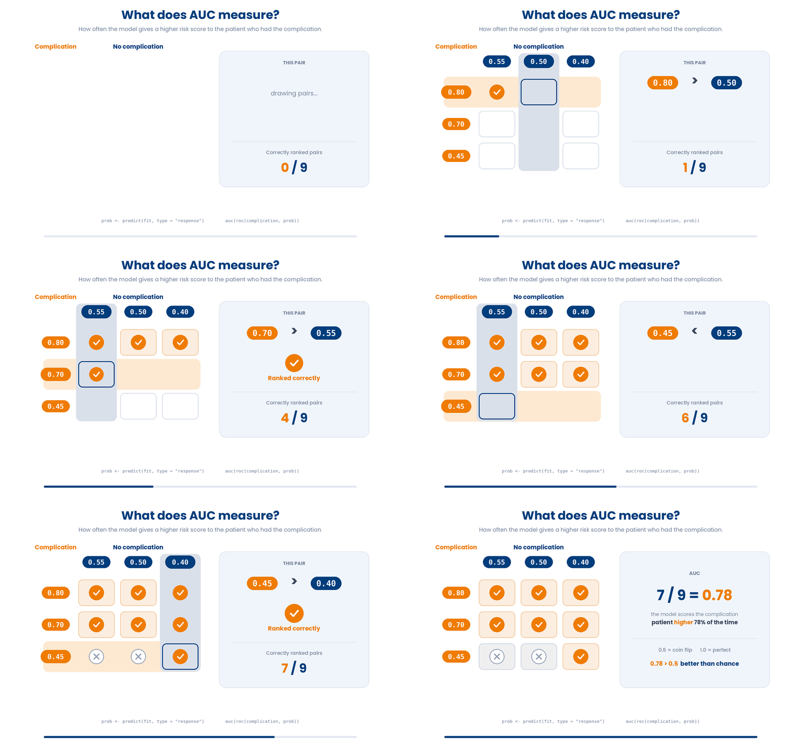
These probabilities let you close the loop with the diagnostics module. A good model gives higher probabilities to patients who actually had the event. We measure that separation — called discrimination — with a ROC curve and its area under the curve, the AUC. An AUC of 0.5 is a coin flip; 1.0 is perfect; clinical models often land between 0.7 and 0.85.
The pROC package builds the curve. Give roc() the true 0/1 outcome and the predicted probabilities; then auc() reads off the area. Plotting the roc object draws the curve.
Try this snippet in the R Scratchpad on the right.
library(pROC)
set.seed(2025)
n <- 300
age <- round(rnorm(n, mean = 60, sd = 10))
smoker <- rbinom(n, 1, 0.35)
complication <- rbinom(n, 1, 1 / (1 + exp(-(-6 + 0.07 * age + 0.8 * smoker))))
cohort <- data.frame(age, smoker, complication)
fit <- glm(complication ~ age + smoker, family = binomial, data = cohort)
cohort$prob <- predict(fit, type = "response")
roc_obj <- roc(cohort$complication, cohort$prob)
auc(roc_obj)
plot(roc_obj)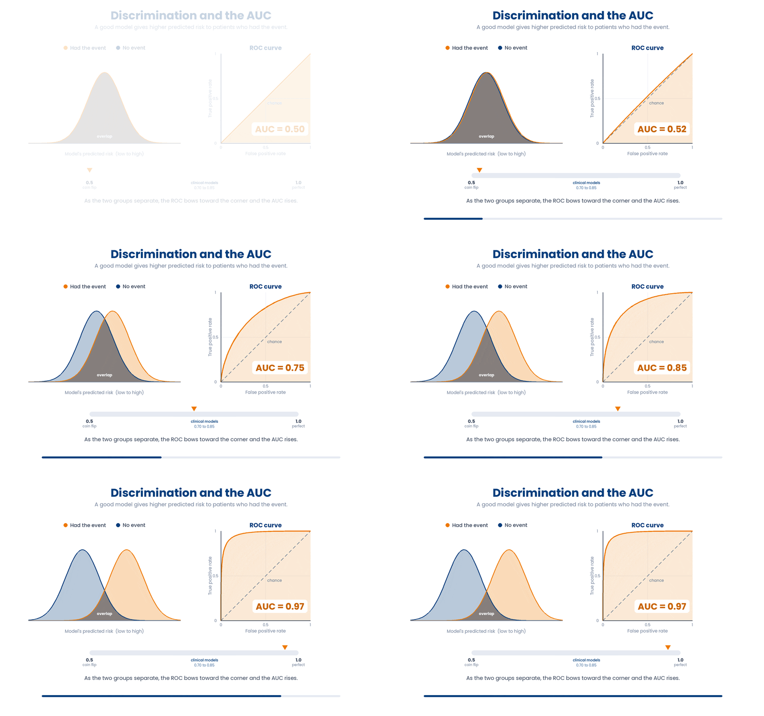
Practise predicting probabilities and scoring them in the example below:
Work through this example in three stages. You unlock each stage only after the tutor confirms the previous one. Each stage removes more of the scaffolding — by the end you are writing it yourself.
Problem: Fit a logistic model, get each patient's predicted probability with predict(type = "response"), and measure discrimination with an ROC AUC.
library(pROC)
set.seed(2025)
age <- round(rnorm(100, 60, 10))
complication <- rbinom(100, 1, plogis(-6 + 0.1 * age))
fit <- glm(complication ~ age, family = binomial)
prob <- predict(fit, type = "response")
auc(roc(complication, prob))- predict(type = "response") gives probabilities, not log-odds
- roc() compares them to the true outcome
- auc() summarises discrimination
The same solution with key parts replaced by ???.
Fill in every ??? so the code matches the reference,
then ask the tutor to check it.
Your turn: An AUC of 0.5 is chance and 1.0 is perfect. Is 0.78 better than chance? Report 0.78 > 0.5.
4 A taste of survival analysis
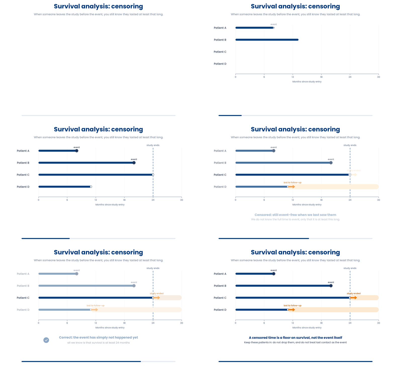
Sometimes the question is not whether an event happens, but when. How long until relapse, until discharge, until death? That is survival analysis, and it needs its own tools because of one feature: censoring.
A patient is censored when the study ends, or they are lost to follow-up, before the event happens. You know they survived at least that long, but not their full time to event. You cannot just drop censored patients or treat their last-seen time as the event time — both throw away real information and bias the result.
4.1 Building the outcome with Surv()
The survival package packs time and status into one outcome with Surv(time, event). The second argument is the event indicator: 1 marks that the event happened; 0 marks a censored observation.
Here is the trap that silently ruins survival analyses. If you code the event indicator backwards — 0 for the event and 1 for censored — every result inverts and no error warns you. Always confirm that 1 = event before you trust a curve.
We will use lung, a cohort of advanced lung-cancer patients that ships inside the survival package. Its time column is survival in days and its status column codes 1 for censored and 2 for dead, so we recode death to a clean 1.
Try this snippet in the R Scratchpad on the right.
library(survival)
lung$died <- ifelse(lung$status == 2, 1, 0)
lung$surv <- Surv(lung$time, lung$died)
head(lung$surv)
A plus sign next to a time in the printed Surv object marks a censored patient. A bare number marks a patient who had the event. That little plus is your visual check that censoring was coded the right way round.
4.2 The Kaplan-Meier curve
The Kaplan-Meier curve estimates the probability of surviving past each time point, stepping down as events occur and accounting for censoring along the way. You fit it with survfit() and a formula whose right side is the grouping — use ~ 1 for the whole cohort, or ~ sex to split by a group.
This course plots survival curves with ggsurvfit. You pass the survfit() object to ggsurvfit() and get a ggplot you can style. Do not reach for survminer — this course standardises on ggsurvfit, and mixing the two only creates confusion.
Try this snippet in the R Scratchpad on the right.
library(survival)
library(ggsurvfit)
lung$died <- ifelse(lung$status == 2, 1, 0)
km_fit <- survfit(Surv(time, died) ~ sex, data = lung)
ggsurvfit(km_fit)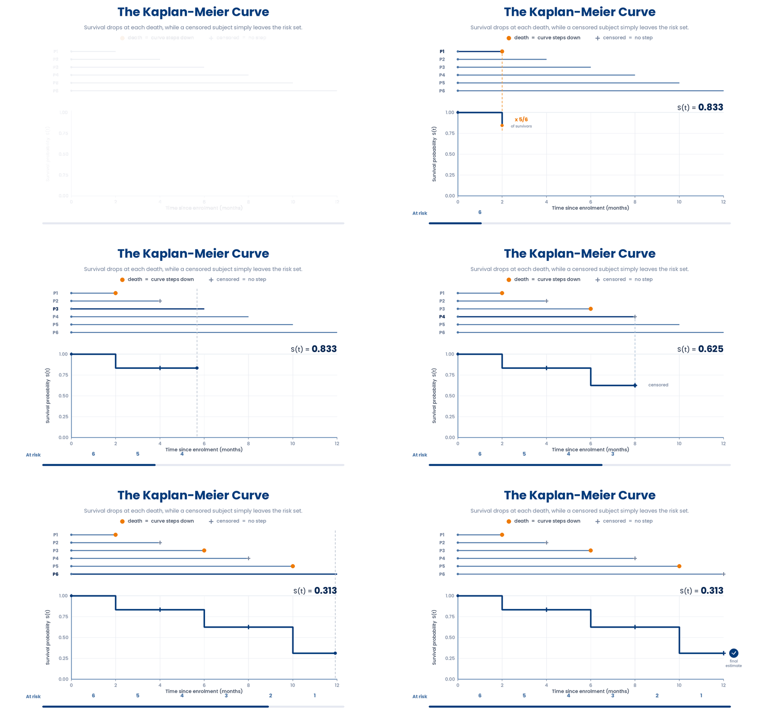
Read the curve at two kinds of landmark. The median survival is the time where the curve crosses 0.5 — half the group has had the event by then. A landmark estimate reads survival at a fixed time, say the one-year probability. Printing the survfit object reports the median for each group.
Try this snippet in the R Scratchpad on the right.
library(survival)
lung$died <- ifelse(lung$status == 2, 1, 0)
km_fit <- survfit(Surv(time, died) ~ sex, data = lung)
km_fit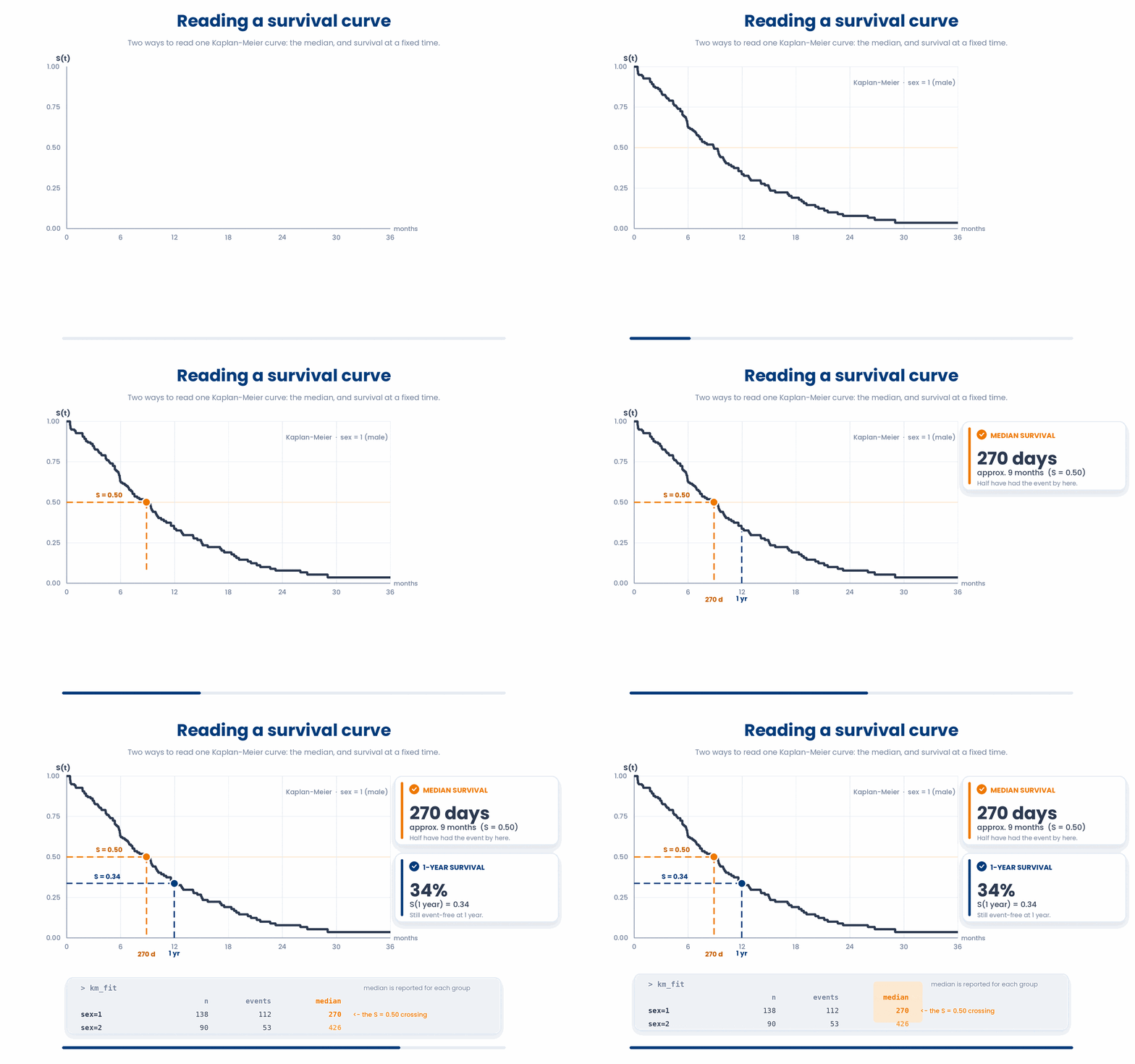
4.3 Comparing two groups: the log-rank test
To ask whether two survival curves differ, use the log-rank test. It compares the observed events in each group with what you would expect if the groups shared one survival curve, and returns a p-value. In R it is survdiff(), with the same Surv() ~ group formula.
Try this snippet in the R Scratchpad on the right.
library(survival)
lung$died <- ifelse(lung$status == 2, 1, 0)
survdiff(Surv(time, died) ~ sex, data = lung)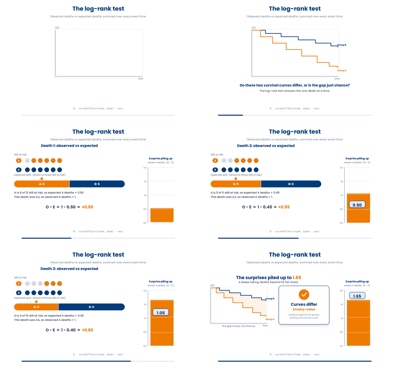
A small p-value says the curves differ more than chance would explain — one group survives longer. But the log-rank test only answers whether they differ, not by how much, and it cannot adjust for other variables the way your logistic model did.
That is where this taste stops. To estimate how much risk differs, adjusted for age and stage, you need Cox proportional-hazards regression and its hazard ratios — the survival cousin of the odds ratio. Cox regression and hazard ratios are deferred to Course 2; survival needs them because the log-rank test compares groups but cannot adjust for
We can compare survival between two groups in the example below
Work through this example in three stages. You unlock each stage only after the tutor confirms the previous one. Each stage removes more of the scaffolding — by the end you are writing it yourself.
Problem: Using the lung dataset, recode death to 1, fit Kaplan-Meier curves split by sex, and test the difference with the log-rank test.
library(survival)
lung$died <- ifelse(lung$status == 2, 1, 0)
km_fit <- survfit(Surv(time, died) ~ sex, data = lung)
survdiff(Surv(time, died) ~ sex, data = lung)- recode status so 1 = death
- survfit() builds the Kaplan-Meier curves by sex
- survdiff() runs the log-rank test for a difference
The same solution with key parts replaced by ???.
Fill in every ??? so the code matches the reference,
then ask the tutor to check it.
Your turn: Re-run the log-rank test split by sex and read the chi-squared p-value it reports.

5 Check your understanding
You have reached the end of the module. Try the same questions again — your answers here, paired with your pre-test answers, are how we measure what the module taught you. Answer every question and confidence rating, then click Submit and see results to view your score.
You have a fitted logistic model fit and want each patient's estimated probability of the event. Which call returns probabilities rather than log-odds?
You run predict(fit) on a logistic model without setting type. What scale are the returned values on?
A colleague reports that their prediction model has an AUC of 0.50. How should you read that?
Which pair of calls measures a logistic model's discrimination, given the true 0/1 outcome and the predicted probabilities?
A patient reaches the end of the study still alive, so their time to death is unknown. In survival analysis this observation is described as
The lung dataset codes its status column as 1 = censored and 2 = dead. Before building a Surv() outcome, why must you recode it so 1 = event?
Which function estimates the Kaplan-Meier survival curve, split by treatment group?
A log-rank test comparing survival in two arms returns p = 0.002. What may you conclude?
I can generate predicted probabilities from a logistic model with predict(type = "response") and explain why the default returns log-odds instead.
I can measure a model's discrimination by building an ROC curve with roc() and reading its AUC, and I know that 0.5 is a coin flip and 1.0 is perfect.
I can code a censored time-to-event outcome with Surv(time, event), draw a Kaplan-Meier curve, and compare two groups with the log-rank test via survdiff() while knowing its limits.
6 Your results
Here is how your post-test answers compare with your pre-test answers. The pre/post pairing is the most reliable way to see what this module actually taught you.
Submit the post-test to see your results.
What is the one thing from this module that is still unclear to you?