Statistical Modeling — Part III: Logistic Regression

Before you begin, take a few minutes to check what you already know and how confident you feel. You will see the same questions again at the end of the module — this helps both you and us measure what you have learned. Click an option for every question and confidence rating, then click Next to continue.

In Part I you fit a linear model with lm() to predict a number — a patient's blood pressure, their HbA1c. But much of clinical research asks a yes/no question instead: did the patient develop a complication, respond to treatment, survive the admission? This part teaches you to model that kind of outcome and report it in the language a clinician actually reads: the odds ratio.

This part of the module covers five skills, built one rung at a time:

• Binary outcomes — recognise a 0/1 outcome, see why a straight line predicts impossible probabilities, and reach for a model built for proportions instead.
• Logistic regression — fit a model for a yes/no outcome with glm(family = binomial) and read its log-odds coefficients.
• Odds ratios — turn the model's coefficients into adjusted odds ratios with exp(), and read one against the line of no effect at 1.
• Publication tables — produce tidy, reportable output with broom::tidy() and gtsummary::tbl_regression().
• Clinical interpretation — put it together: fit the model, exponentiate, and state one adjusted odds ratio and its confidence interval in plain clinical words.

By the end of this part you will be able to fit a logistic regression, explain why a 0/1 outcome needs glm(family = binomial) rather than lm(), convert its coefficients to adjusted odds ratios and interpret one for a clinician, and produce a tidy, publication-ready table of odds ratios with 95% confidence intervals.

Try every snippet in the R Scratchpad on the right. This part needs no data file — the examples build a small simulated cohort of 300 surgical patients with set.seed(), so everyone who runs the code gets the exact same cohort.

Part I predicted a continuous number, so lm() was the right tool. Now the outcome is binary — it takes exactly two values, coded 0 and 1, such as 0 for no complication and 1 for a complication. Averaging a 0/1 column gives you the proportion with the event, which is a probability between 0 and 1.

The classic novice trap is to fit lm() to that 0/1 column as if it were a number. A straight line is not bounded between 0 and 1, so it happily predicts a probability of 1.3 or minus 0.2 — impossible values. The fix is a model built for proportions.

That model is logistic regression. You fit it with glm() — the generalised linear model function — and you tell it the outcome is binary by setting family = binomial. The glm part is base R, from the stats package that is always loaded.

Let us build a small cohort to model. We simulate 300 patients whose risk of a post-operative complication rises with age and is higher in smokers. Using set.seed() first means everyone who runs this code gets the exact same cohort.

set.seed(2025)
n <- 300
age <- round(rnorm(n, mean = 60, sd = 10))
smoker <- rbinom(n, 1, 0.35)
lp <- -6 + 0.07 * age + 0.8 * smoker
prob <- 1 / (1 + exp(-lp))
complication <- rbinom(n, 1, prob)
cohort <- data.frame(age, smoker, complication)
mean(cohort$complication)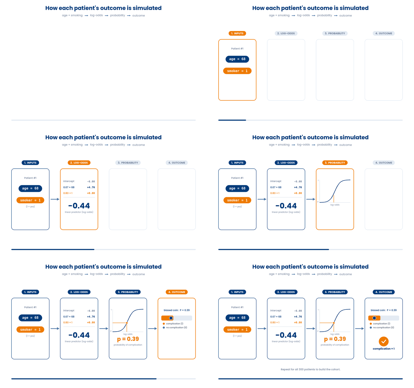

Notice the last line: mean() of a 0/1 column is the event rate — the proportion of patients who had a complication. That single number is what a logistic model explains in terms of age and smoking.

With the cohort in hand, the model fits in one line. The formula reads outcome on the left, predictors on the right, joined by a tilde: complication ~ age + smoker. The + means you adjust for both predictors at once.

set.seed(2025)
n <- 300
age <- round(rnorm(n, mean = 60, sd = 10))
smoker <- rbinom(n, 1, 0.35)
lp <- -6 + 0.07 * age + 0.8 * smoker
complication <- rbinom(n, 1, 1 / (1 + exp(-lp)))
cohort <- data.frame(age, smoker, complication)
fit <- glm(complication ~ age + smoker, family = binomial, data = cohort)
summary(fit)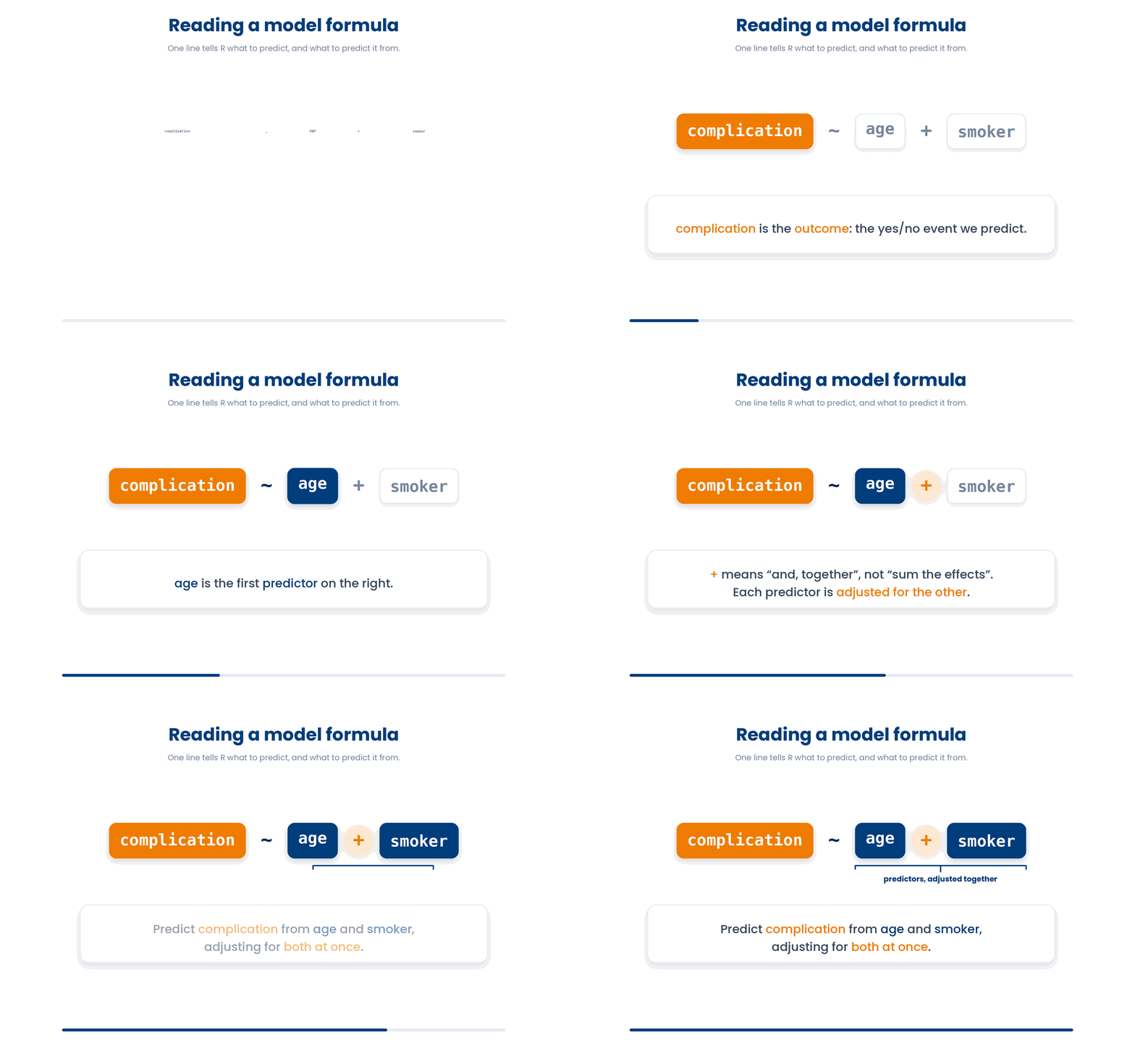

Read the Estimate column of the summary. Each estimate is a log-odds coefficient: the change in the natural log of the odds of a complication for a one-unit rise in that predictor, holding the others fixed. Log-odds are correct but unreadable — nobody thinks in log-odds at the bedside.

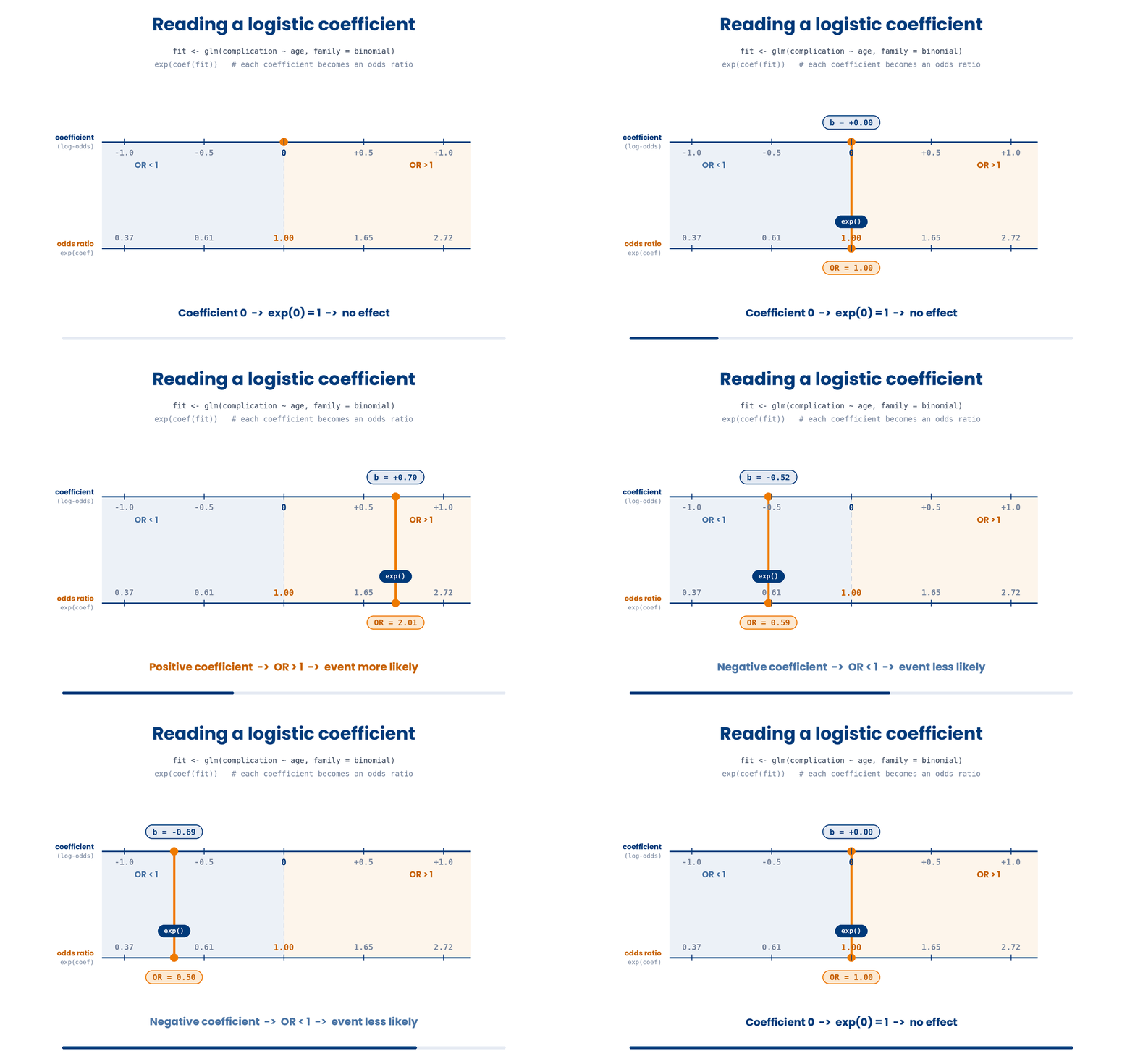
Here is the trap that catches every beginner. On the log-odds scale, a coefficient of 0 means no effect — not 1. A positive coefficient raises the odds; a negative one lowers them. To make the numbers speak, you exponentiate them, which is the next rung.

Let’s try and fit a model built for a yes/no outcome.

age <- c(45, 52, 61, 58, 70, 49, 65, 55)
complication <- c(0, 0, 1, 0, 1, 0, 1, 0)
fit <- glm(complication ~ age, family = binomial)
summary(fit)

The fix for unreadable log-odds is the odds ratio, written OR. You get it by exponentiating a coefficient with exp(). The odds ratio compares the odds of the event in one group to the odds in another, after adjusting for every other predictor in the model.

Read an odds ratio against 1, not 0. An OR above 1 means higher odds of the event; below 1 means lower odds; exactly 1 means no effect. The reference point is 1 because exponentiating the no-effect coefficient of 0 gives exp(0), which is 1.

So forgetting to exponentiate is the cardinal sin of logistic regression. The raw glm coefficient is a log-odds; an OR of 1 — not 0 — is the line of no effect. Always ask whether

Do the exponentiation yourself on the whole model. exp(coef(fit)) turns every log-odds coefficient into an odds ratio at once — the line you reach for after almost every logistic fit.

set.seed(2025)
n <- 300
age <- round(rnorm(n, mean = 60, sd = 10))
smoker <- rbinom(n, 1, 0.35)
complication <- rbinom(n, 1, 1 / (1 + exp(-(-6 + 0.07 * age + 0.8 * smoker))))
cohort <- data.frame(age, smoker, complication)
fit <- glm(complication ~ age + smoker, family = binomial, data = cohort)
exp(coef(fit))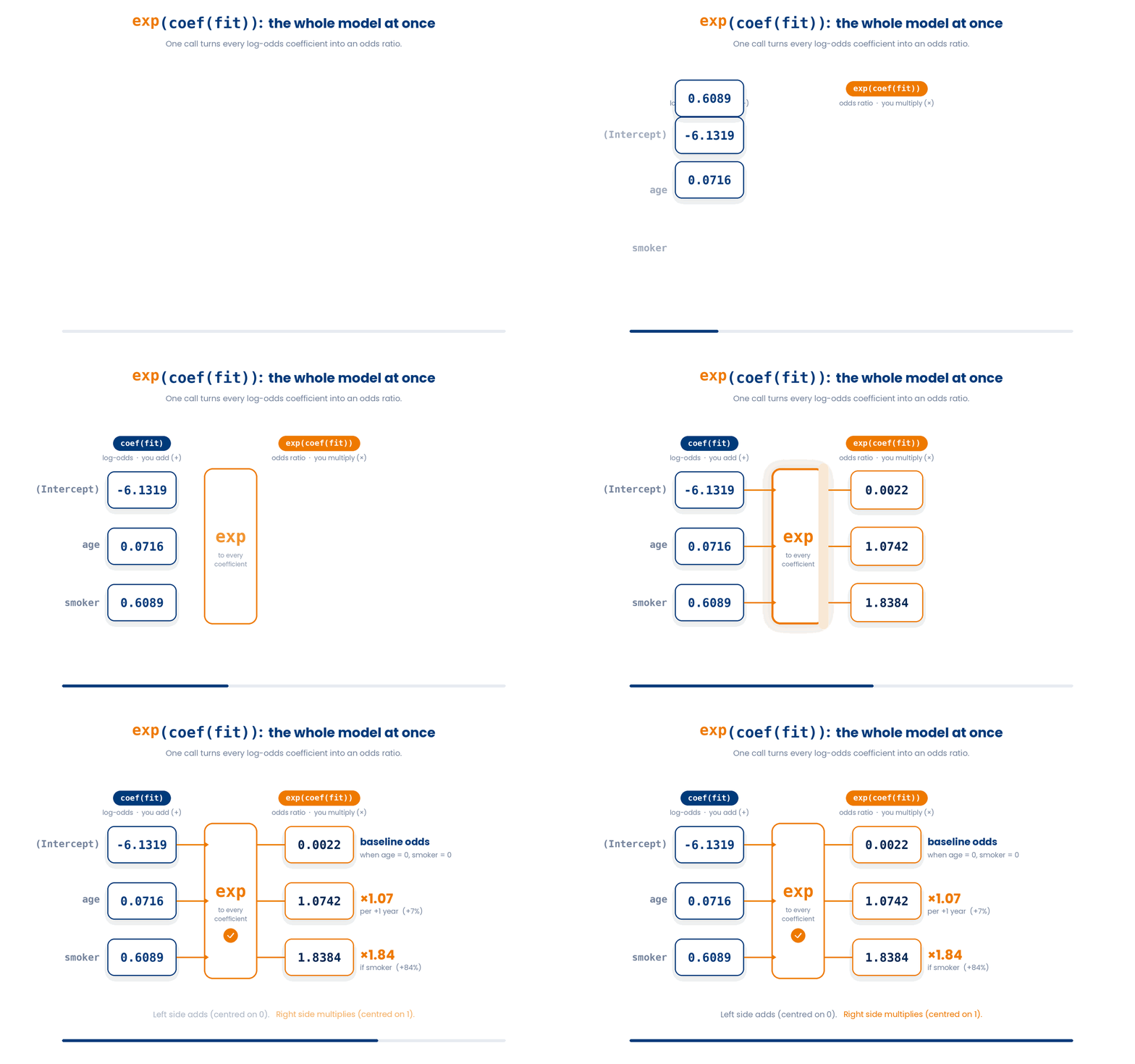

One more distinction students blur. An odds ratio is not a risk ratio. A risk ratio compares probabilities directly; an odds ratio compares odds, where odds are probability divided by one-minus-probability. For a rare outcome the two are close, but for a common outcome an odds ratio is further from 1 than the risk ratio — never report an OR as if it were a relative risk.

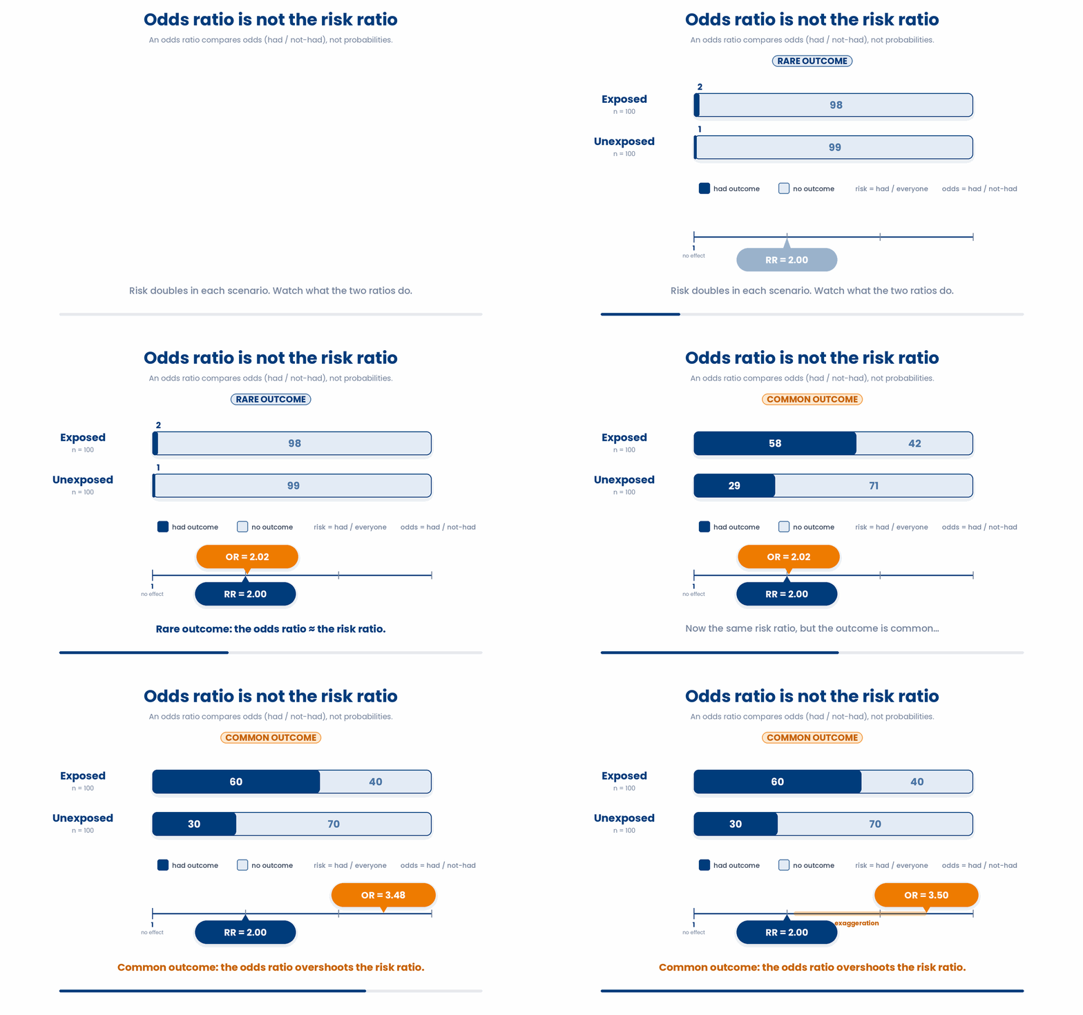
Let’s practise turn a log-odds into a readable odds ratio.

coef_smoker <- 0.8
round(exp(coef_smoker), 2)

Reading odds ratios off a summary() by hand is slow and error-prone. Two packages turn the model into a clean table. First, broom tidies any model into a data frame you can sort, filter, and reuse.

Call broom::tidy() with exponentiate = TRUE to report odds ratios instead of log-odds, and conf.int = TRUE to add a 95% confidence interval. The :: writes the package name before the function, so you can see exactly where it comes from.

library(broom)
set.seed(2025)
n <- 300
age <- round(rnorm(n, mean = 60, sd = 10))
smoker <- rbinom(n, 1, 0.35)
complication <- rbinom(n, 1, 1 / (1 + exp(-(-6 + 0.07 * age + 0.8 * smoker))))
cohort <- data.frame(age, smoker, complication)
fit <- glm(complication ~ age + smoker, family = binomial, data = cohort)
tidy(fit, exponentiate = TRUE, conf.int = TRUE)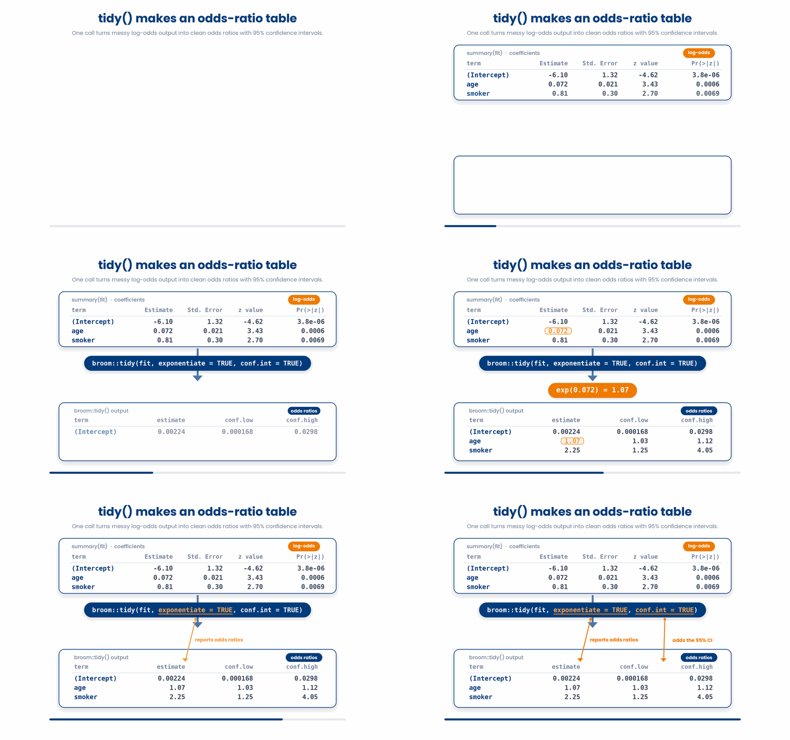

For a table you can paste straight into a manuscript, reach for gtsummary. Its tbl_regression() function takes the fitted model and, with exponentiate = TRUE, prints adjusted odds ratios with confidence intervals and p-values, already formatted with proper variable labels.

library(gtsummary)
set.seed(2025)
n <- 300
age <- round(rnorm(n, mean = 60, sd = 10))
smoker <- rbinom(n, 1, 0.35)
complication <- rbinom(n, 1, 1 / (1 + exp(-(-6 + 0.07 * age + 0.8 * smoker))))
cohort <- data.frame(age, smoker, complication)
fit <- glm(complication ~ age + smoker, family = binomial, data = cohort)
tbl_regression(fit, exponentiate = TRUE)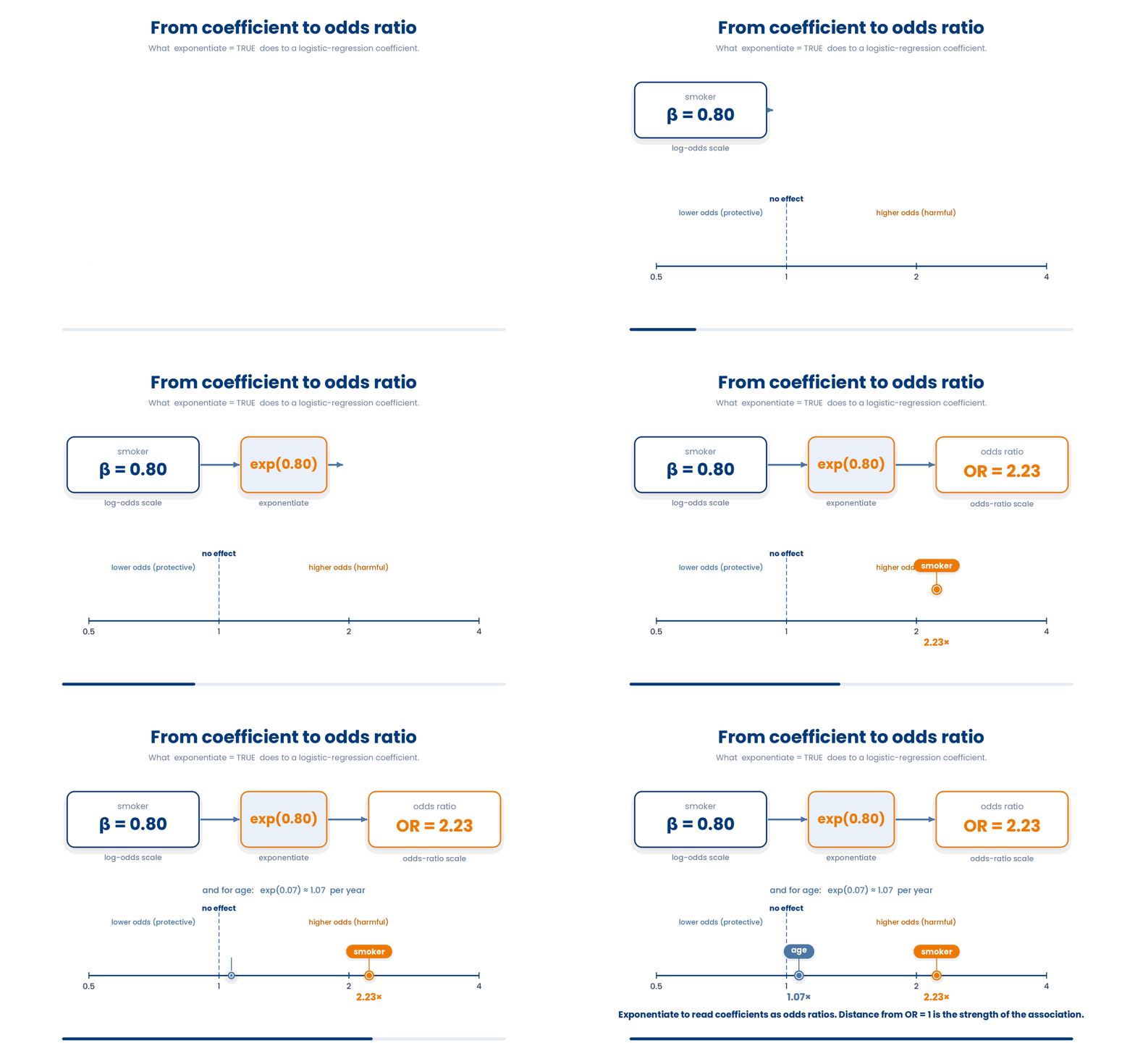

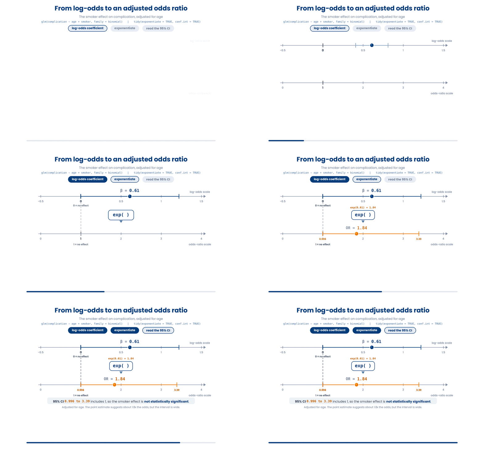
Now interpret one odds ratio in plain clinical language. Suppose the adjusted OR for smoker is 2.1, with a 95% confidence interval of 1.2 to 3.7. You would write: after adjusting for age, smokers have about 2.1 times the odds of a post-operative complication compared with non-smokers, and the interval excludes 1, so the association is statistically significant.

The worked example below fades the support as you go: first you study a full solution, then you fill the gap, then you solve a fresh one on your own. The core skill is fitting a logistic model and reporting an adjusted odds ratio.

library(broom)
set.seed(2025)
n <- 300
age <- round(rnorm(n, mean = 60, sd = 10))
smoker <- rbinom(n, 1, 0.35)
complication <- rbinom(n, 1, 1 / (1 + exp(-(-6 + 0.07 * age + 0.8 * smoker))))
cohort <- data.frame(age, smoker, complication)
fit <- glm(complication ~ age + smoker, family = binomial, data = cohort)
tidy(fit, exponentiate = TRUE, conf.int = TRUE)

You have reached the end of the module. Try the same questions again — your answers here, paired with your pre-test answers, are how we measure what the module taught you. Answer every question and confidence rating, then click Submit and see results to view your score.

Here is how your post-test answers compare with your pre-test answers. The pre/post pairing is the most reliable way to see what this module actually taught you.