Statistical Modeling — Part I: Correlation and Fitting a Line

Before you begin, take a few minutes to check what you already know and how confident you feel. You will see the same questions again at the end of the module — this helps both you and us measure what you have learned. Click an option for every question and confidence rating, then click Next to continue.

In Module 6 you compared groups — you asked whether two arms of a trial differ. Now you ask a richer question: as one measurement changes, how does another change with it? Modelling a relationship lets you say not just THAT HbA1c rises with age, but by how much per year. This part takes you from a first look at how two measurements move together to a fitted straight line whose slope you can read off and hand to a clinician.

This part of the module covers three foundations that build on one another:

• Correlation — a single number from -1 to +1 that summarises how two measurements move together, measured with cor() and tested with cor.test().
• Simple linear regression — the single best straight line through the cloud of points, fitted with lm() and the formula outcome ~ predictor.
• Reading the model — pulling the slope, intercept, and R-squared out of summary() and interpreting the slope in clinical units.

By the end of this part you will be able to measure and test a correlation between two continuous measurements, fit a simple linear regression with lm(), and read its slope, intercept, and R-squared from summary() — stating the slope in real clinical units and knowing which numbers are safe to interpret and which are not.

Try every snippet in the R Scratchpad on the right. This part needs no data file — you will build a small cohort with set.seed(), c(), and data.frame() so everyone sees the same numbers. Use the native pipe |> if you reach for a pipe.

Before you fit any line, you take a first look at whether two measurements move together at all. Correlation gives you that look as a single number, and it is where every regression story starts.

A correlation — strictly, the Pearson correlation coefficient, written r — measures the strength and direction of the STRAIGHT-LINE relationship between two continuous measurements. It runs from -1 to +1. A value near +1 means they rise together; near -1 means one falls as the other rises; near 0 means no straight-line relationship.

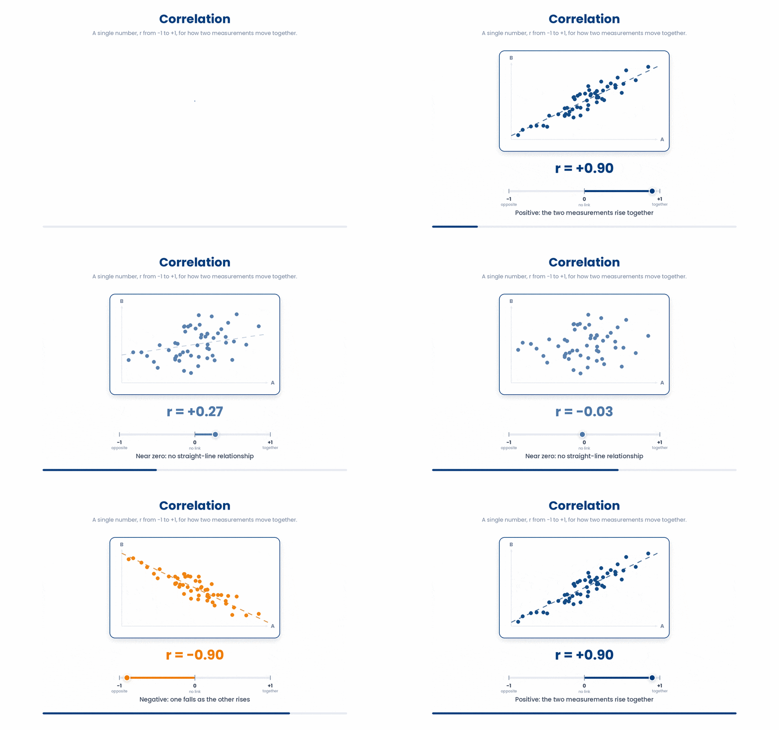
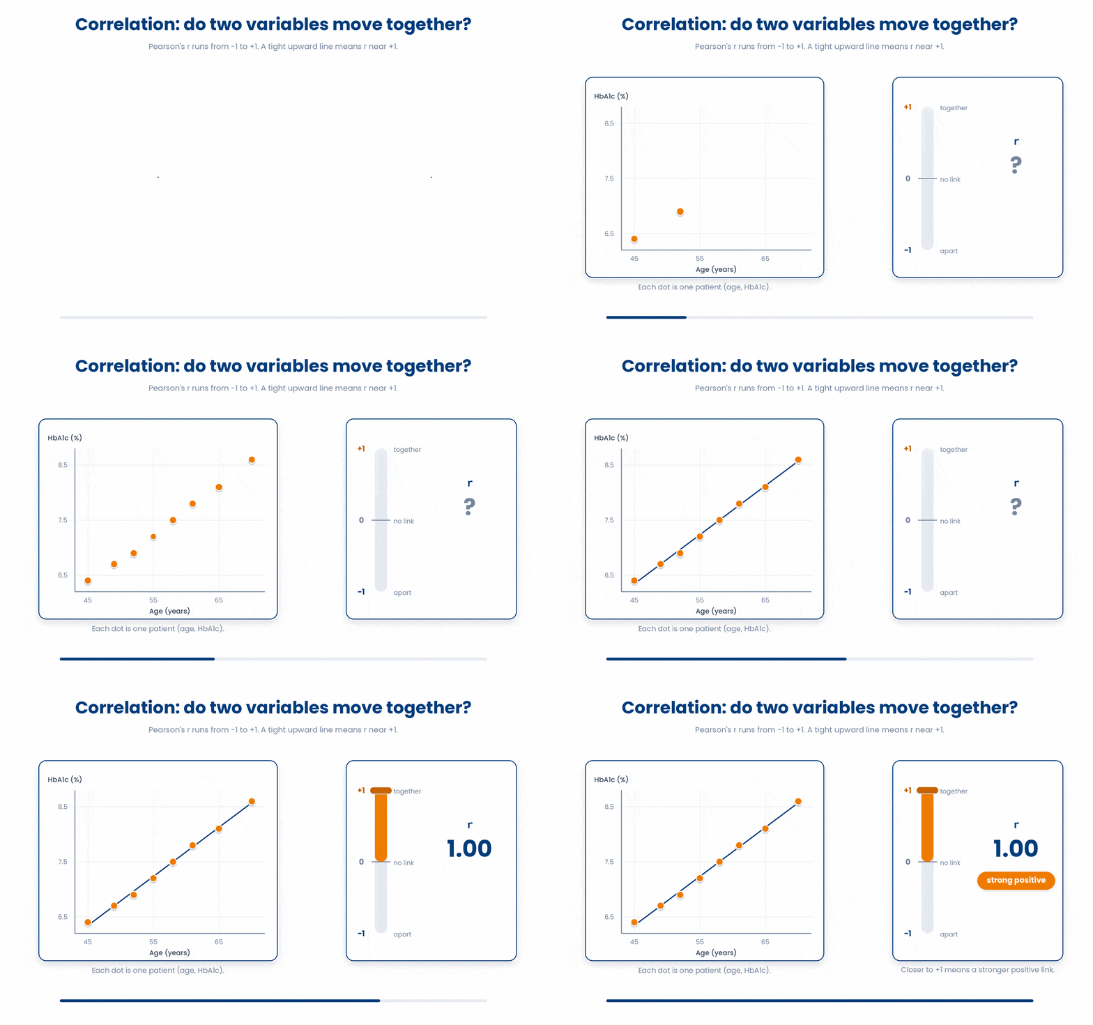
Make it concrete. In a diabetes clinic you suspect that older patients tend to have higher HbA1c. You measure age and HbA1c on a handful of patients and ask R for the correlation with cor(). A value of, say, 0.7 says they move together fairly strongly and in the same direction.

age <- c(45, 52, 61, 58, 70, 49, 65, 55)
hba1c <- c(6.4, 6.9, 7.8, 7.5, 8.6, 6.7, 8.1, 7.2)
cor(age, hba1c)

Read the sign first, then the size. A positive r means the two go up together; a negative r means one goes down as the other goes up. As a rough clinical guide, an r around 0.1 is weak, 0.3 is moderate, and 0.5 or more is strong — but the thresholds always depend on the field.

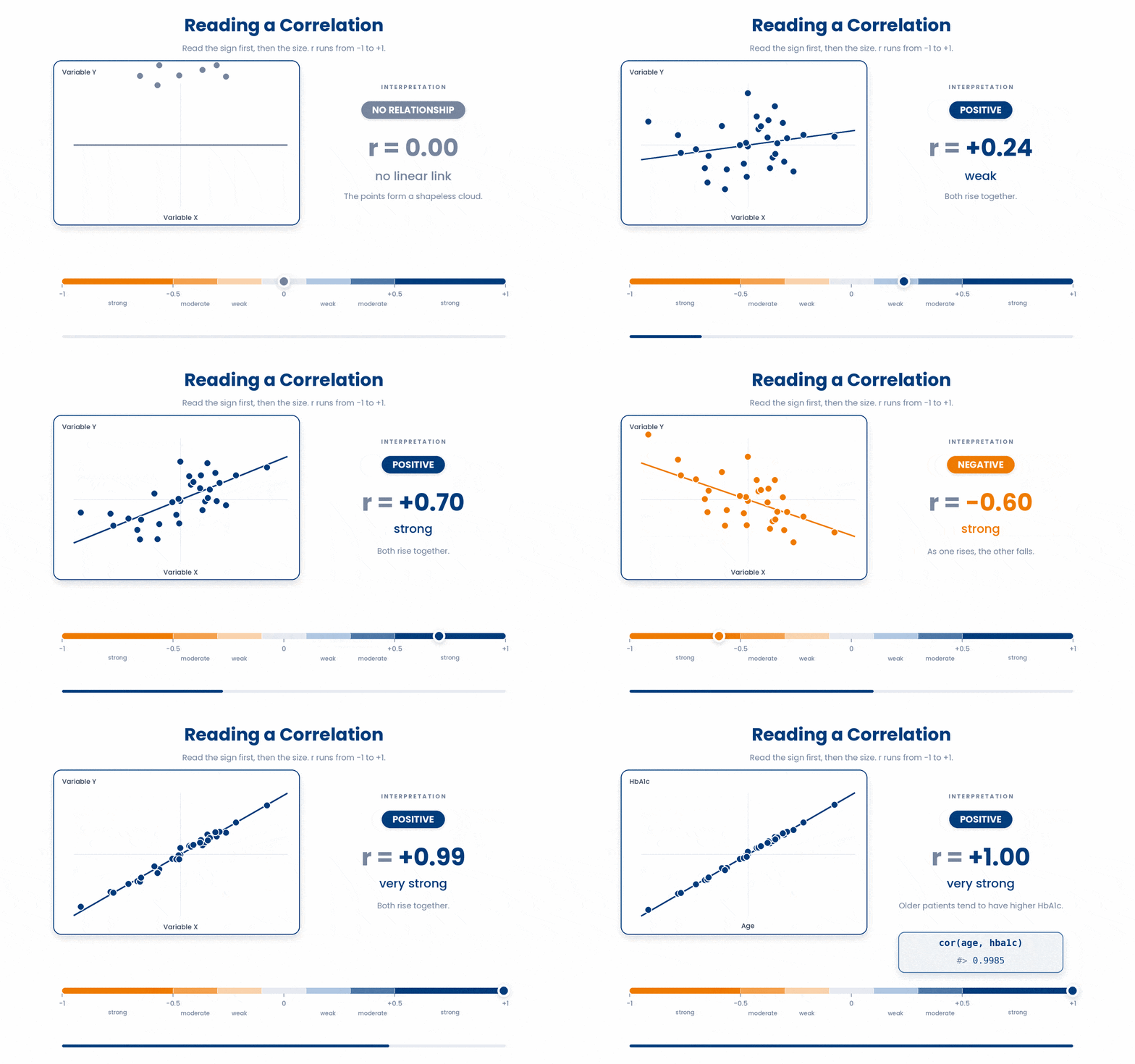
A perfect straight line gives r exactly 1 or exactly -1. You can see this with toy numbers: if y

Here is the trap that has launched a thousand bad headlines. A correlation, however strong, is not proof that one thing causes the other. Ice-cream sales correlate with drownings, but ice cream does not drown anyone — summer heat drives both. Correlation tells you two things move together; it never tells you why.

cor() gives you the number; cor.test tells you whether it is more than noise. It reports the same r, plus a p-value testing whether the true correlation differs from zero, and a 95% confidence interval for r. Use it when you want to know if an apparent association could be a chance pattern in a small sample.

Run it on the same age and HbA1c. The printout names the correlation under "cor" and gives the interval and p-value above it. Put it in the scratchpad and read the whole block.

age <- c(45, 52, 61, 58, 70, 49, 65, 55)
hba1c <- c(6.4, 6.9, 7.8, 7.5, 8.6, 6.7, 8.1, 7.2)
cor.test(age, hba1c)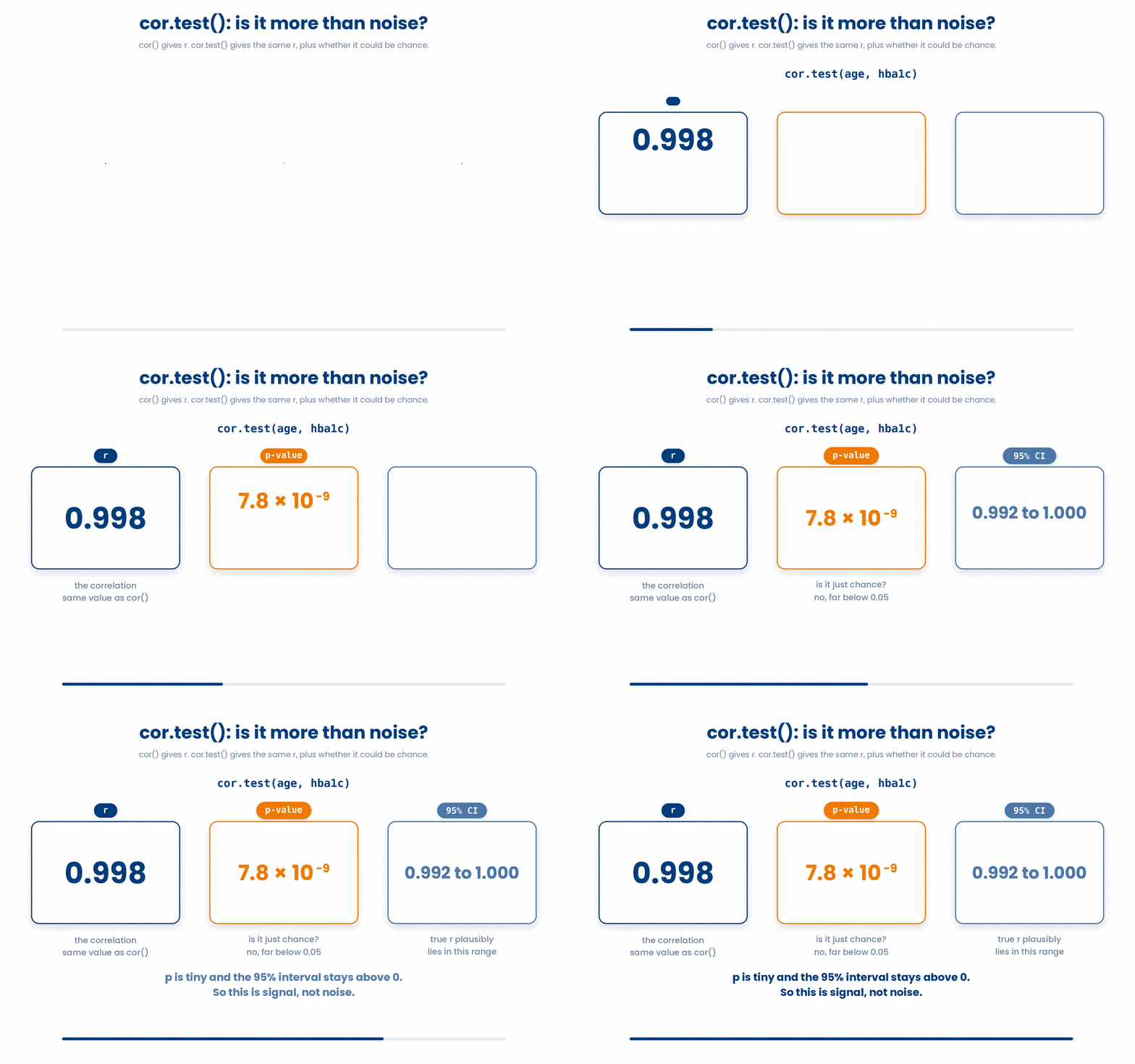

One scope note before you go further. cor() measures only a STRAIGHT-LINE association. Two variables can have a strong curved relationship and still show a correlation near zero — so always look at a scatterplot, never the number alone. You will draw that scatterplot in Section 4.

Let’s measure how two variables move together.

age <- c(45, 52, 61, 58, 70, 49, 65, 55)
hba1c <- c(6.4, 6.9, 7.8, 7.5, 8.6, 6.7, 8.1, 7.2)
round(cor(age, hba1c), 2)

Correlation tells you two measurements move together and how tightly. Regression goes one step further: it draws the actual line, so you can say how much the outcome changes for each unit of the predictor.

A simple linear regression fits the single best straight line through a cloud of points. The line has the form outcome = intercept + slope * predictor. The outcome (also called the response or dependent variable) is what you want to explain; the predictor (the explanatory or independent variable) is what you use to explain it.

By "best" line R means the least-squares line: the one line that makes the vertical gaps between the points and the line as small as possible, squared and summed. Each gap — the difference between a patient's actual outcome and the line's prediction — is called a residual.

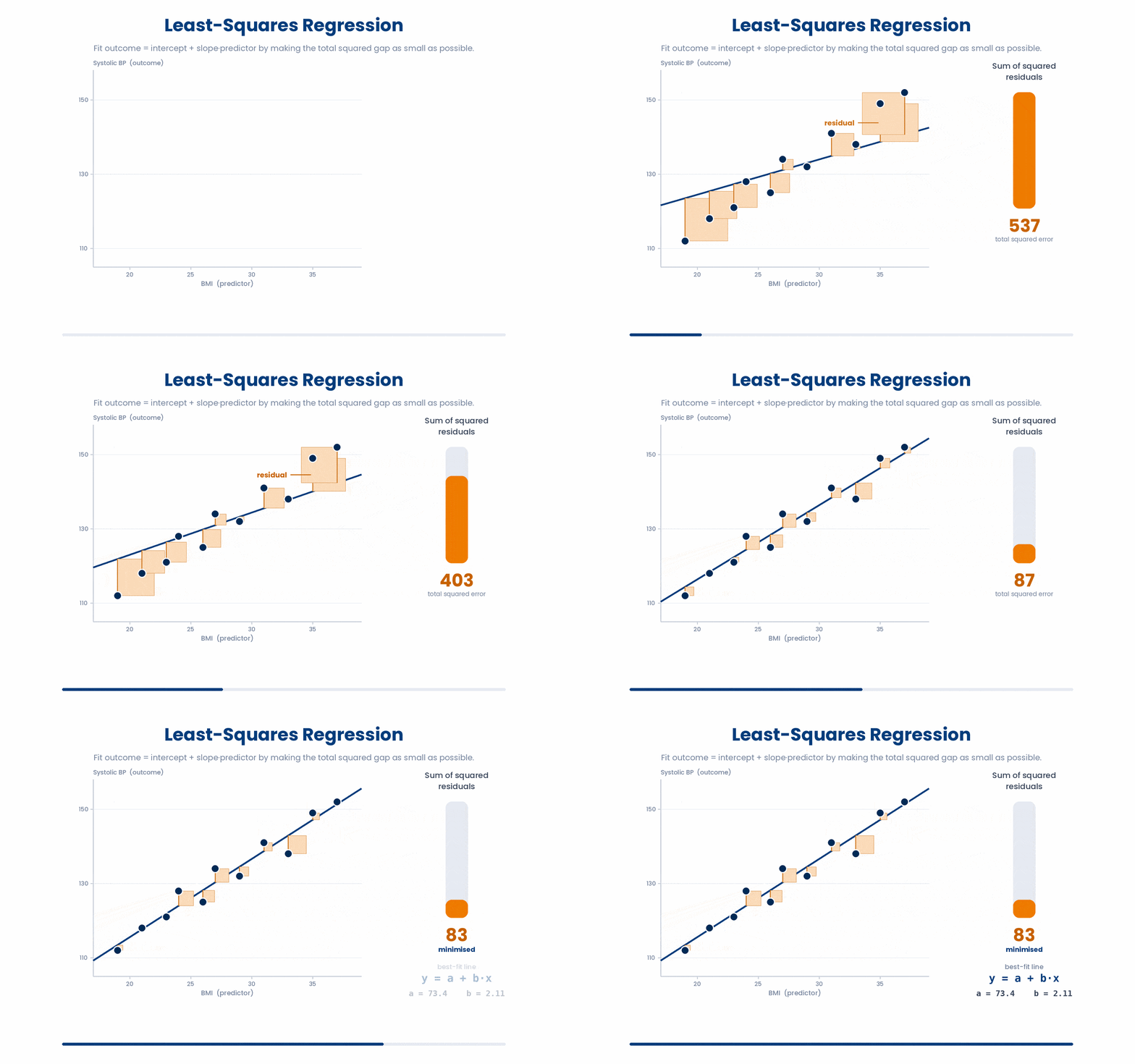
You fit it with lm (for linear model) using R's formula interface: lm(outcome ~ predictor, data = your_data). Read the tilde ~ as "is modelled by" or "depends on". So hba1c ~ age means "model HbA1c as a function of age".

Build a small, reproducible cohort first. set.seed() fixes the random numbers so your results match everyone else's. Here HbA1c rises with age plus some noise, exactly the kind of data regression is built for.

set.seed(123)
age <- round(rnorm(40, mean = 60, sd = 8))
hba1c <- 4 + 0.05 * age + rnorm(40, mean = 0, sd = 0.4)
clinic <- data.frame(age, hba1c)
model <- lm(hba1c ~ age, data = clinic)
model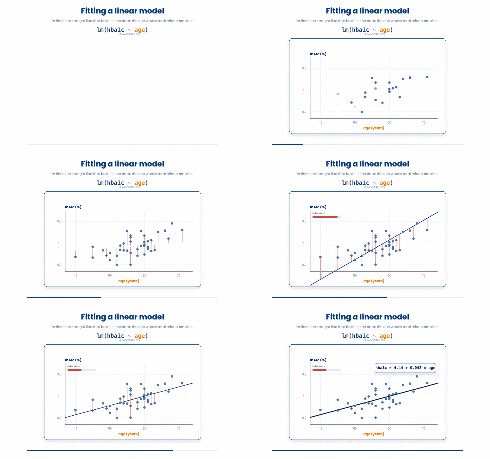

Mind the order in the formula. The outcome goes on the LEFT of the tilde and the predictor on the RIGHT. Writing lm(age ~ hba1c) fits a completely different model — it tries to predict age from HbA1c. Always put the thing you want to explain first.

When you print a fitted model, R shows the Coefficients: the intercept and the slope for age. Those two numbers ARE the line. The next section reads them properly. First, lock in the formula direction with this small fix.

You have a fitted line, but a bare model object hides most of what you need. The function that opens it up is summary(), and learning to read its output is the heart of this whole part.

Call summary on the model and you get a table with one row per coefficient. The (Intercept) row and the age row each give an Estimate, a standard error, a t-value, and a p-value. The Estimate column holds the two numbers that define your line.

set.seed(123)
age <- round(rnorm(40, mean = 60, sd = 8))
hba1c <- 4 + 0.05 * age + rnorm(40, mean = 0, sd = 0.4)
clinic <- data.frame(age, hba1c)
model <- lm(hba1c ~ age, data = clinic)
summary(model)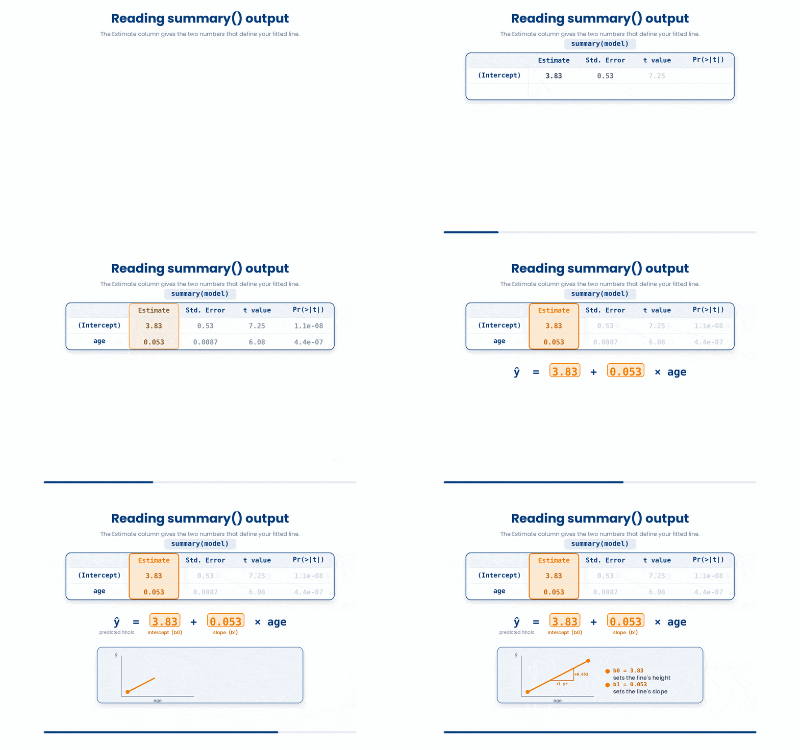

The slope is the Estimate on the age row, and it is the single most useful number in the model. It says how much the outcome changes for a ONE-UNIT increase in the predictor. If the age slope is 0.05, then each extra year of age is associated with an HbA1c that is 0.05 percentage points higher, on average. Always state the slope in real clinical units like this.

The intercept is the Estimate on the (Intercept) row: the predicted outcome when the predictor is exactly zero. Here that is the predicted HbA1c for a patient of age zero — a newborn — which is clinically meaningless. Do not interpret an intercept when zero is impossible or absurd for the predictor; it is only there to position the line.

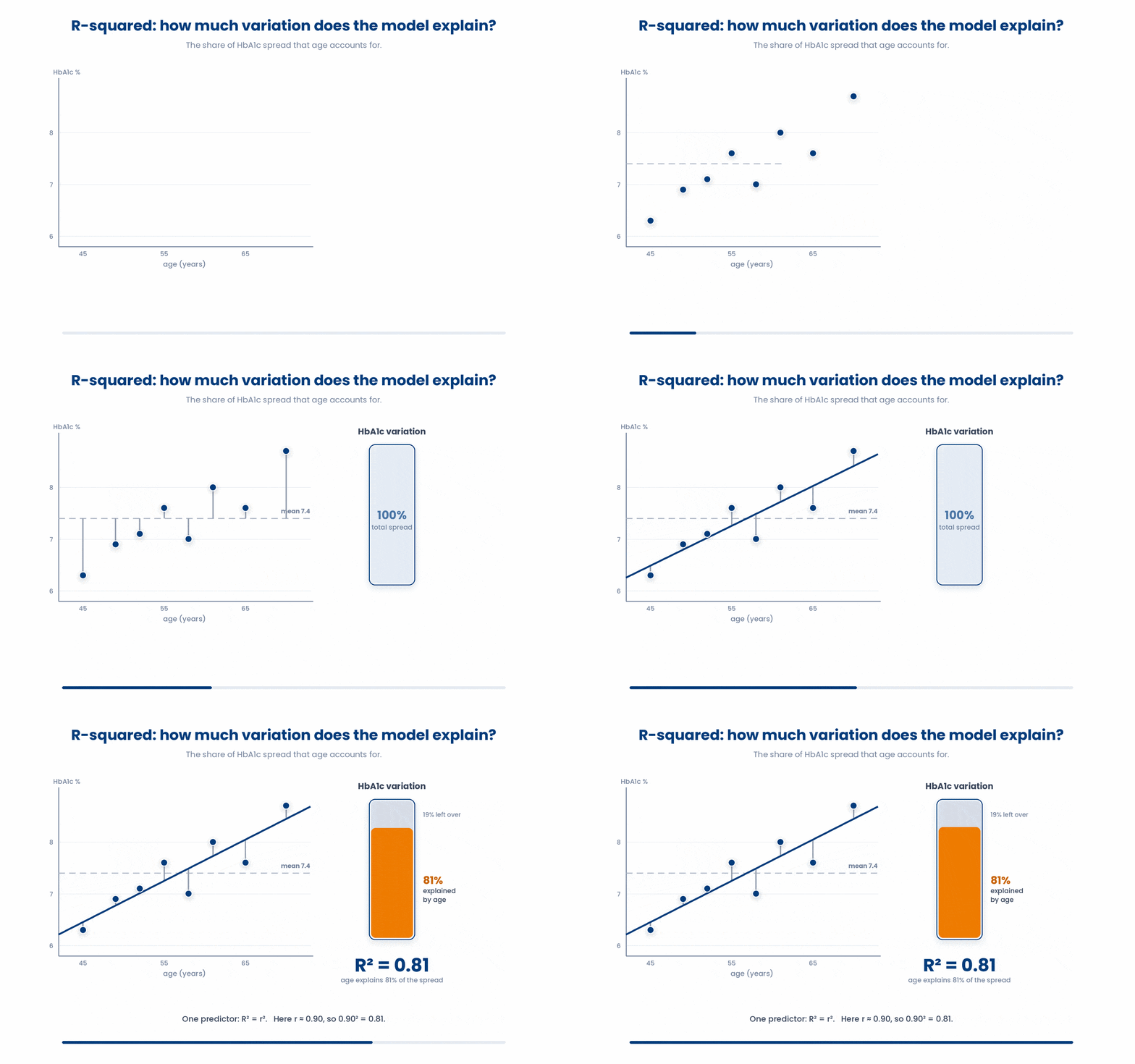
The R-squared — shown near the bottom as "Multiple R-squared" — is the proportion of the variation in the outcome that the model explains, from 0 to 1. An R-squared of 0.30 means age accounts for 30% of the spread in HbA1c; the remaining 70% is other things and noise. For a single predictor it is simply the correlation squared.

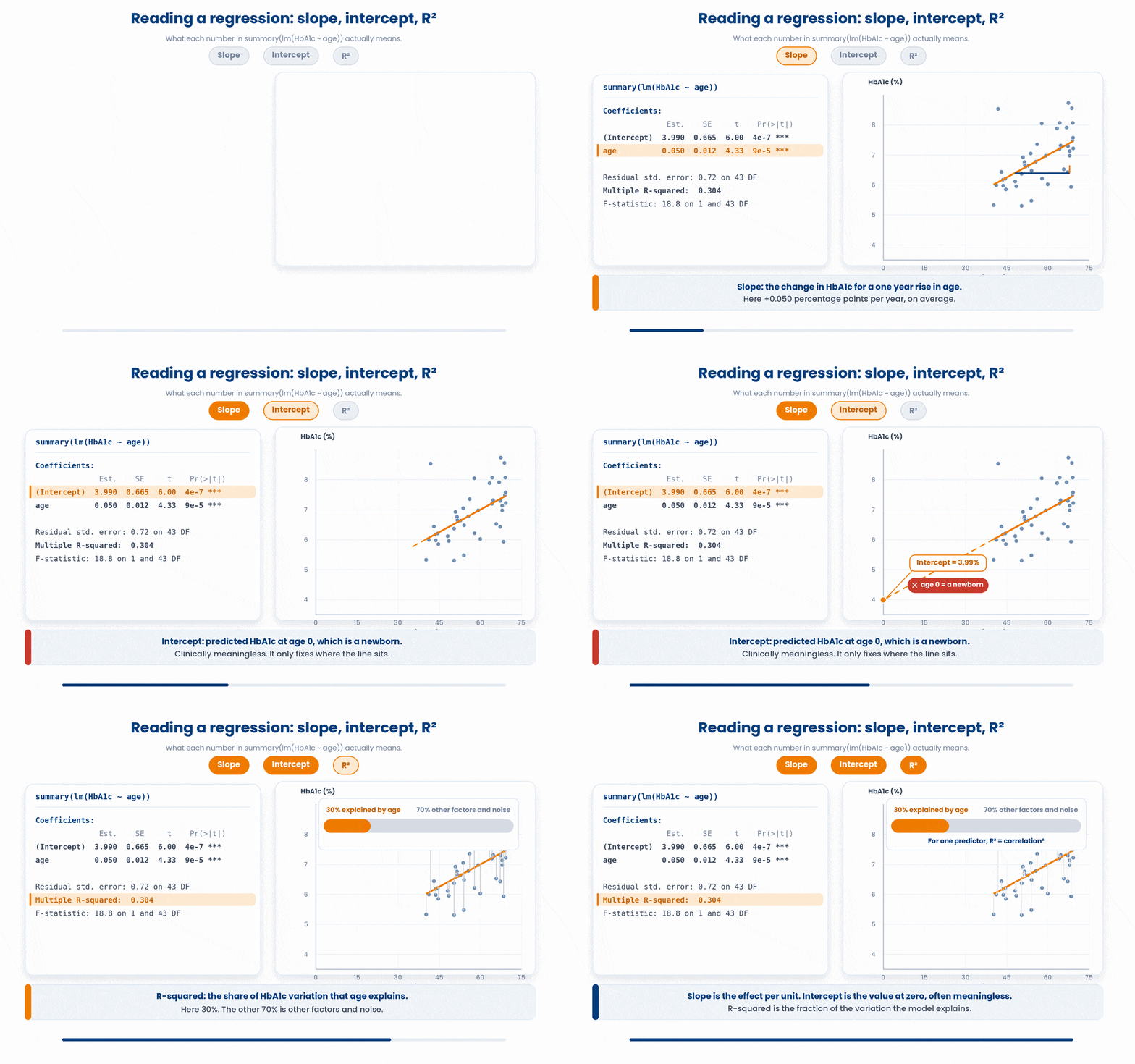
A common misread: treating a high R-squared as proof the model is correct or that age CAUSES the change. R-squared measures how much variation is explained, not whether the relationship is causal or the model is right. A model can fit tightly and still be the wrong model.

Let’s read how much variation the model explains.

age <- c(45, 52, 61, 58, 70, 49, 65, 55)
hba1c <- c(6.4, 6.9, 7.8, 7.5, 8.6, 6.7, 8.1, 7.2)
model <- lm(hba1c ~ age)
round(summary(model)$r.squared, 2)

You have reached the end of the module. Try the same questions again — your answers here, paired with your pre-test answers, are how we measure what the module taught you. Answer every question and confidence rating, then click Submit and see results to view your score.

Here is how your post-test answers compare with your pre-test answers. The pre/post pairing is the most reliable way to see what this module actually taught you.