Effect Measures and ROC — Part I: Multiple Testing and Effect Measures

Before you begin, take a few minutes to check what you already know and how confident you feel. You will see the same questions again at the end of the module — this helps both you and us measure what you have learned. Click an option for every question and confidence rating, then click Next to continue.

In the hypothesis-testing module a test gave you a yes/no answer and a p-value. That is only half the story. Running one test is safe; running twenty is where false positives creep in. And once a test is significant, a clinician still needs the size of the effect — how much more likely is the outcome in one group than another? This part turns that concern into two skills: keeping false positives under control across a family of tests, and turning the four counts of a 2x2 table into the effect measures that papers actually report.

This part of the module covers three foundations, each feeding the next:

• The multiple-testing problem — why running many tests inflates false positives, and fixing it with p.adjust() using the Benjamini-Hochberg and Bonferroni methods.
• Effect measures from a 2x2 table — the odds ratio, relative risk, risk difference, and number-needed-to-treat, each with a confidence interval, read straight off the counts with epiR::epi.2by2().
• Which design yields which measure — a cohort or RCT gives you real risk, so relative risk, risk difference, and NNT; a case-control study gives you an odds ratio only.

By the end of this part you will be able to adjust a family of p-values for multiple testing with p.adjust() and read an adjusted p-value against alpha, read an odds ratio, relative risk, risk difference, and NNT with their confidence intervals from a 2x2 table, and say which of those measures a given study design actually supports.

Try every snippet in the R Scratchpad on the right. This part needs no data file — you will build a small vector of p-values with c() and a 2x2 table with matrix(). Use the native pipe |> if you reach for a pipe, and call library() explicitly for every package so it pre-installs.

Before we measure effects, fix a danger that grows the moment you run more than one test. Part I set alpha at 0.05 — a 5% false-alarm rate per test. That budget is per test, and it does not survive being spent many times.

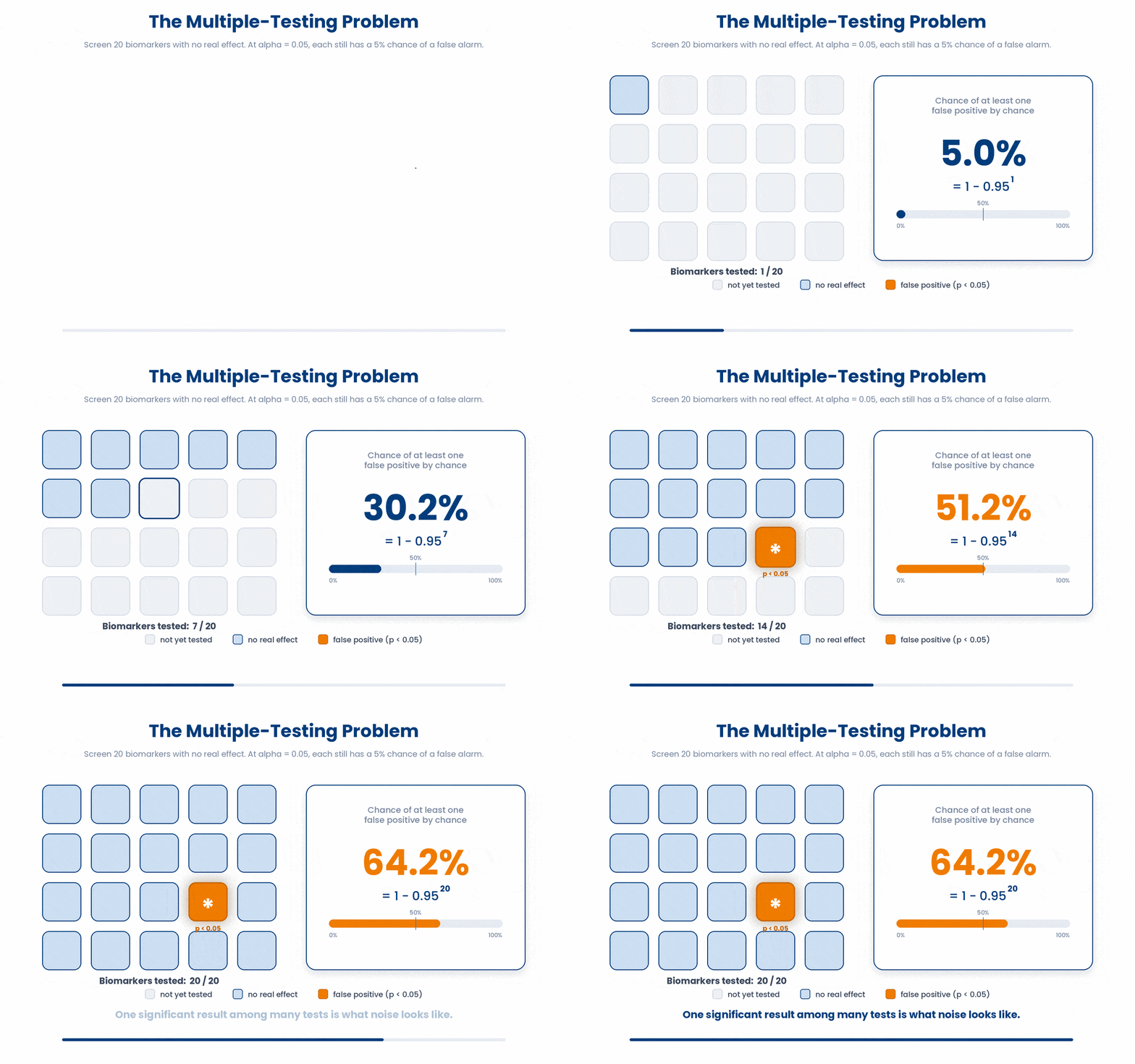
The multiple-testing problem is this: every test you run carries its own 5% chance of a false positive, so running many tests almost guarantees at least one. Test 20 truly-null biomarkers at alpha 0.05 and you expect one to look significant by chance alone.

Make it concrete. You screen 20 biomarkers for a link to diabetes, and none truly matters. The chance that at least one crosses p < 0.05 by luck is 1 - 0.95^20, about 64%. So a single significant p-value out of many tests is not evidence on its own — it is what you would expect from noise.

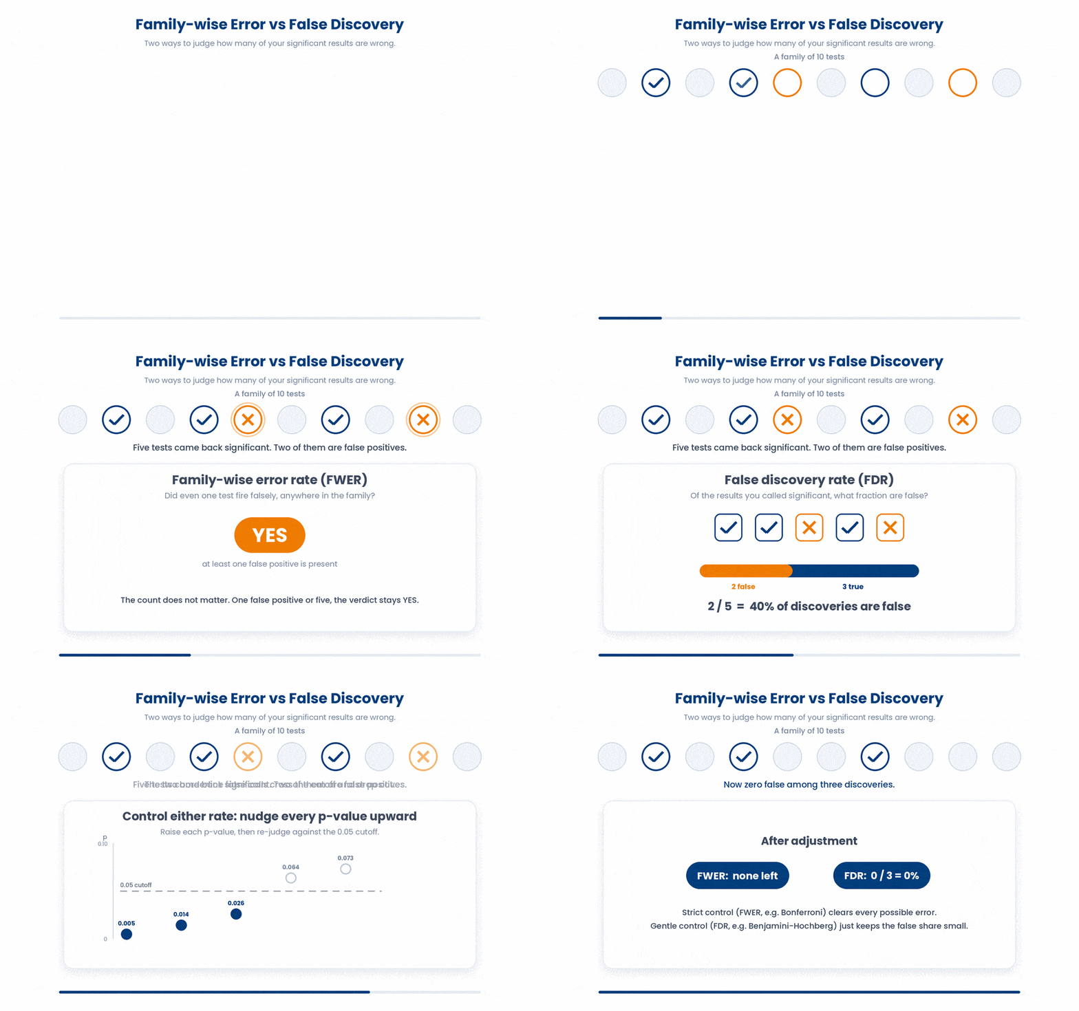
The family-wise error rate is the chance of making even one false positive across the whole family of tests. The false discovery rate — the FDR — is the gentler idea: of the results you call significant, what fraction are false? You control one or the other by adjusting the p-values upward before you judge them.

R adjusts a vector of p-values in one call: p.adjust(). The Bonferroni method is the strict one — it multiplies every p-value by the number of tests, controlling the family-wise error rate. It is safe but conservative, so it can hide real effects.

The Benjamini-Hochberg method — written method = "BH" — controls the false discovery rate instead. It is less harsh than Bonferroni, so it keeps more power, and it is the default choice for a small family of clinical tests. Pass your raw p-values and the method name.

pvals <- c(0.001, 0.02, 0.04, 0.30, 0.80)
p.adjust(pvals, method = "BH")
p.adjust(pvals, method = "bonferroni")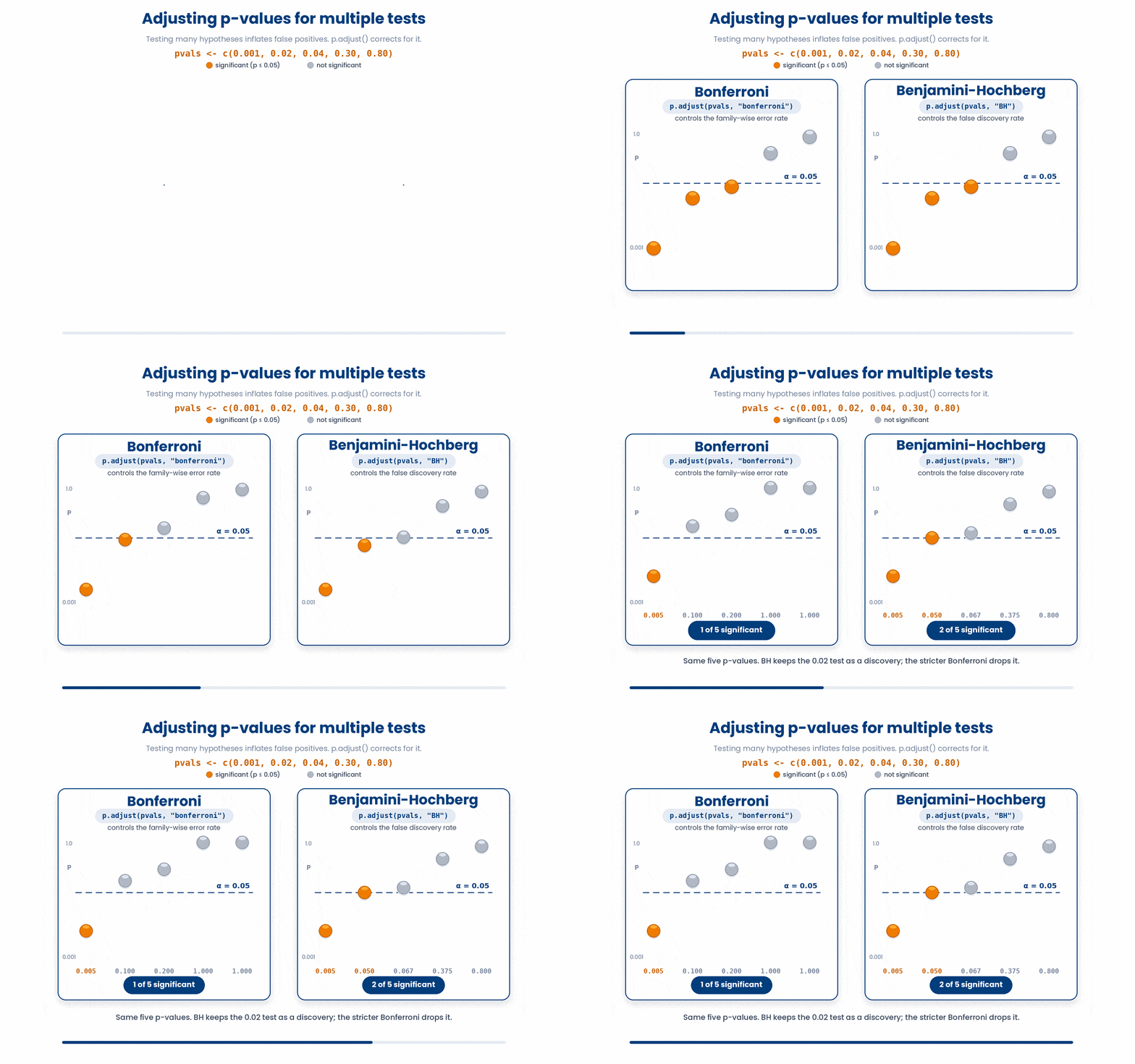

Read the output the right way. An adjusted p-value is compared against your original alpha (0.05), not against itself or some new threshold. You still ask: is the ADJUSTED p below 0.05? Some raw p-values that passed will now fail — that is the whole point.

One scope note. This hand-sized family of five tests is the everyday case. Omics-scale FDR — thousands of genes at once — is Course 2; the BH method here is the same engine those pipelines use, just on a small vector.

With the multiple-testing guard in place, turn to the effect itself. When the outcome is binary — disease or no disease — you cross-tabulate it against exposure into a two-by-two table, and read several measures from those four counts.

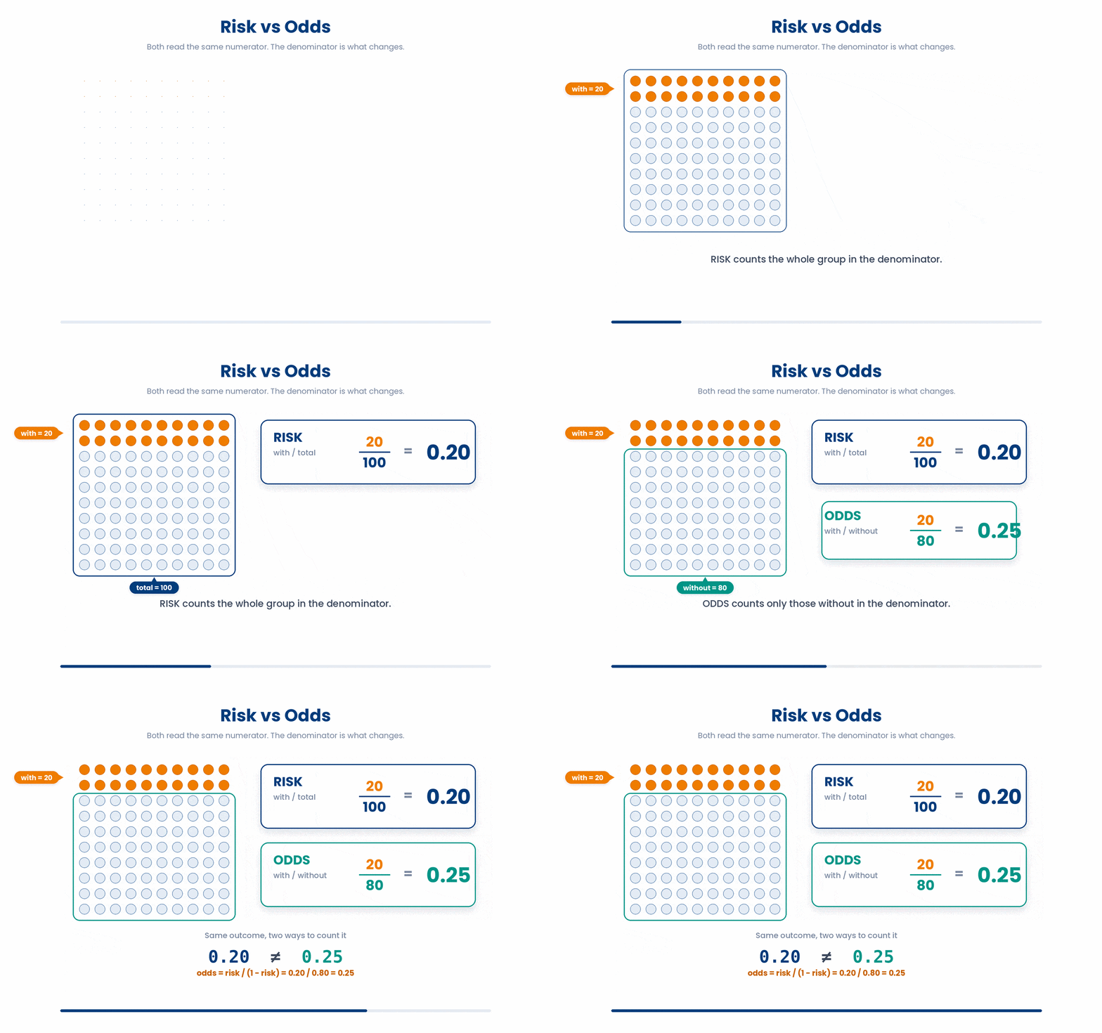
First, two words you must not blur. The risk of an outcome is its probability: the number with the outcome divided by the total in that group. The odds of an outcome is the number with it divided by the number without it. A risk of 0.20 is the same event as odds of 0.20 / 0.80, which is 0.25 — the two numbers differ.

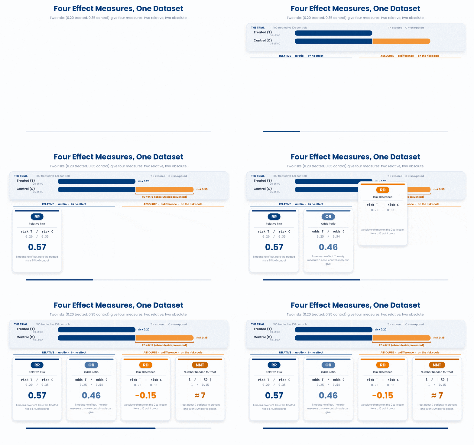
From the four counts you read four effect measures:

• relative risk (RR) — the risk in the exposed divided by the risk in the unexposed. RR = 1 means no effect; RR = 2 means the exposed have twice the risk.
• odds ratio (OR) — the odds in the exposed divided by the odds in the unexposed. OR = 1 means no effect; it is the only measure a case-control study can give.
• risk difference (RD) — the risk in the exposed minus the risk in the unexposed, an absolute change on the same 0-to-1 scale.
• number-needed-to-treat (NNT) — 1 / |RD|, how many patients you must treat to prevent one extra event. Small is good.

Make it concrete. In a trial, 20 of 100 treated patients have a heart attack versus 35 of 100 controls. The risk is 0.20 treated, 0.35 control. The risk difference is 0.20 - 0.35 = -0.15: treatment cuts absolute risk by 15 points. The NNT is 1 / 0.15, about 7 patients treated per event prevented.

You rarely compute these by hand. The epiR package takes the 2x2 table and returns every measure WITH a confidence interval and the right test. The key is feeding it the table in the order it expects: exposed row first, outcome-present column first.

Build the table with explicit factor levels so the order is never left to chance. If you let R sort the levels alphabetically, it can flip the rows or columns and report the reciprocal of the measure you wanted. Set the levels yourself, then eyeball the printed table to confirm the counts sit where you expect.

library(epiR)
dat <- matrix(c(20, 80, 35, 65), nrow = 2, byrow = TRUE)
rownames(dat) <- c("Treated", "Control")
colnames(dat) <- c("MI", "No MI")
dat
epi.2by2(dat, method = "cohort.count")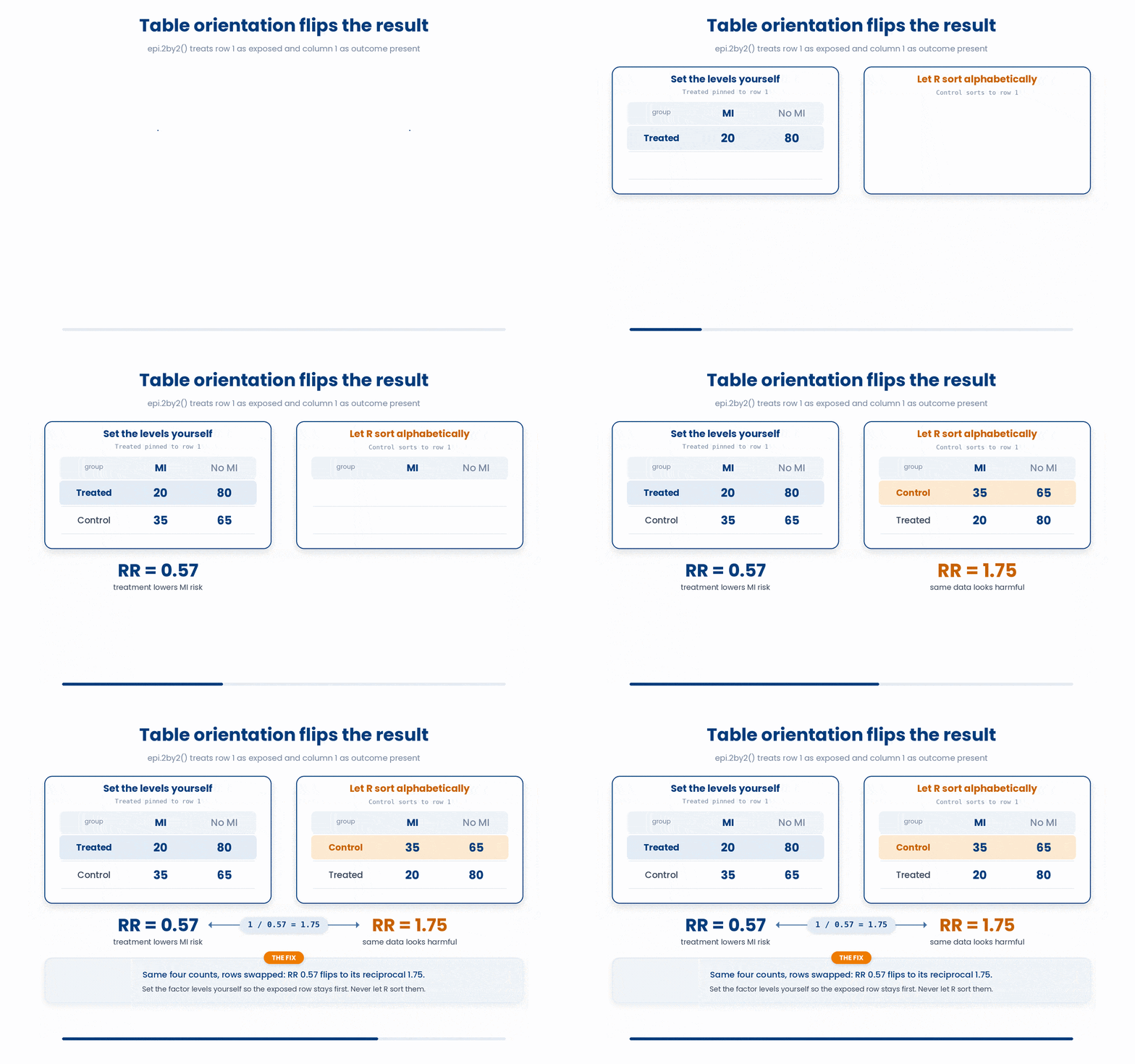

Read the printout in clinical words: an Inc risk ratio is the relative risk, Odds ratio is the OR, Attrib risk is the risk difference, and NNT appears in the same block. Each comes with a 95% CI. A CI that crosses 1 (for RR or OR) or crosses 0 (for RD) means the effect is not significant.

You now have four measures, but you cannot report all of them from every study. The design you ran decides which numbers are even meaningful — and this is where the classic odds-ratio mistake lives.

In a cohort study or a randomised controlled trial (RCT) you start with exposed and unexposed groups and follow them forward, so you can measure the actual risk in each group. That lets you report the relative risk, the risk difference, and the NNT — the measures clinicians find easiest to act on.

In a case-control study you start from the outcome — you pick people who already have the disease and people who do not — then look back at exposure. Because you chose how many cases to enrol, the column totals are fixed by design, so the risks are not real risks. From a case-control study you can report an odds ratio only — never a relative risk or a risk difference.

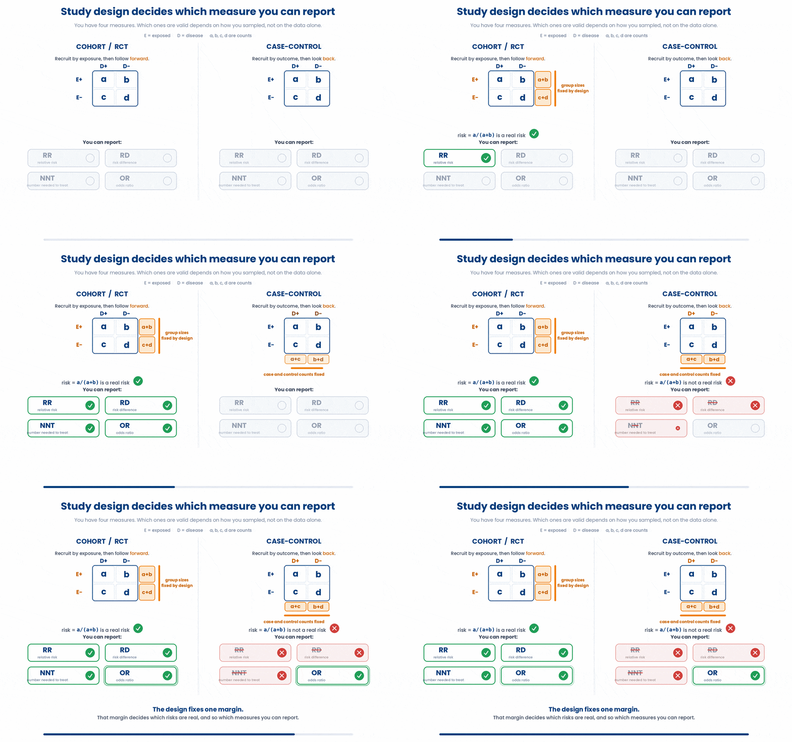
Now the trap that catches everyone. Do not report an odds ratio from a cohort or RCT as if it were a relative risk. When the outcome is common the OR exaggerates the RR — an OR of 2.5 can correspond to an RR of only 1.6. They agree only when the outcome is rare. Say 'odds ratio' when you mean odds ratio.

You have reached the end of the module. Try the same questions again — your answers here, paired with your pre-test answers, are how we measure what the module taught you. Answer every question and confidence rating, then click Submit and see results to view your score.

Here is how your post-test answers compare with your pre-test answers. The pre/post pairing is the most reliable way to see what this module actually taught you.