

1 Before you start
This is not graded, and it does not count towards anything. Answer every question even if you are only guessing — having a go at something before you have been taught it is one of the best ways to remember it afterwards. The lesson ends with another short check, and there you will be shown the correct answer for anything you missed. Choose an option for every question and confidence rating, then click Submit answers.
You set alpha = 0.05 and your test returns p = 0.02. What does alpha represent here?
A regulator rejects a drug's null hypothesis of no effect, but in truth the drug does nothing. Which error is this?
A trial is designed with 80% power to detect a clinically important effect. What does this mean?
An underpowered trial of 8 patients returns a non-significant p-value for a drug that truly works. What most likely happened?
You want the n per group for 80% power to detect Cohen's d of 0.5 at alpha 0.05. Which call solves for it?
You decide to switch to a one-sided test only after seeing the effect points the way you hoped. Why is this a problem?
With 10,000 patients, a mean HbA1c difference of 0.02% reaches p < 0.001. How should you report it?
You compare a continuous, roughly Normal outcome across THREE treatment arms at once. Which test fits?
I can explain alpha, Type I and Type II error, and power in plain clinical words, and say why an underpowered study can miss a real effect.
I can plan a study's sample size with pwr.t.test(), commit to a one-sided or two-sided test before seeing the data, and tell statistical significance from clinical significance.
I can recognise whether data are paired or independent, choose and run the correct base-R test after checking its assumptions, and tidy the result with broom::tidy().
2 Introduction
In Part I you learned to state a null and an alternative, run a test, and read the p-value it returns without the classic misreadings. A p-value alone does not tell you what to do next. This part gives you the rule for acting on it and an honest account of how that rule can fail: the two errors every test can make, the power to catch a real effect, and the choice of which test actually fits your data.
This part of the module covers four foundations, each building toward a defensible decision:
- Errors and power — alpha, Type I and Type II error, and why an underpowered study misses real effects.
- Planning sample size — fixing three of effect size, sample size, alpha, and power, and letting pwr solve for the fourth.
- Significance, two ways — one-sided versus two-sided tests, and statistical versus clinical significance.
- Choosing a test — a decision aid for t.test, aov, wilcox.test, chisq.test and cor.test, the paired-data trap, and checking assumptions.
By the end of this part you will be able to explain alpha, Type I and Type II error, and power in clinical words, plan a sample size with pwr.t.test(), commit to a one-sided or two-sided test honestly, tell statistical from clinical significance, recognise when data are PAIRED rather than independent, and choose and run the correct base-R test, tidying its result with broom::tidy().
Try every snippet in the R Scratchpad on the right. This part needs no data file — you will build small trials with c(), matrix() and set.seed() and let base R run the tests. Use the native pipe |> if you reach for a pipe, and call library() explicitly for every package.
3 Alpha, the two errors, and power
Once you understand the p-value, you need a rule for acting on it, and an honest account of how that rule can fail. Every test can be wrong in two directions, and planning for them happens before you collect a single patient.
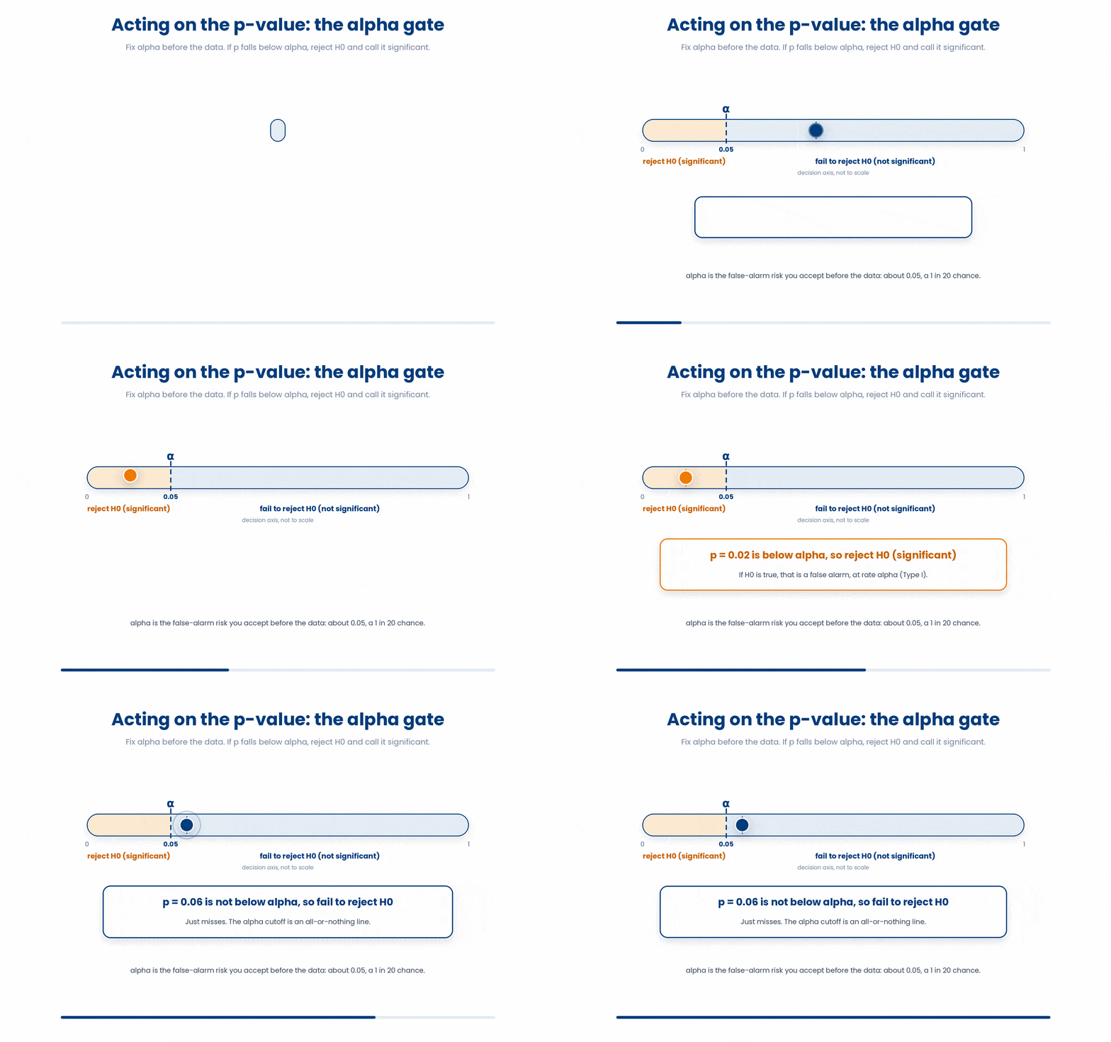
You fix a threshold called alpha — the significance level — before seeing the data, conventionally 0.05. If the p-value falls below alpha you reject H0 and call the result statistically significant. Alpha is the risk you are willing to take of a false alarm.
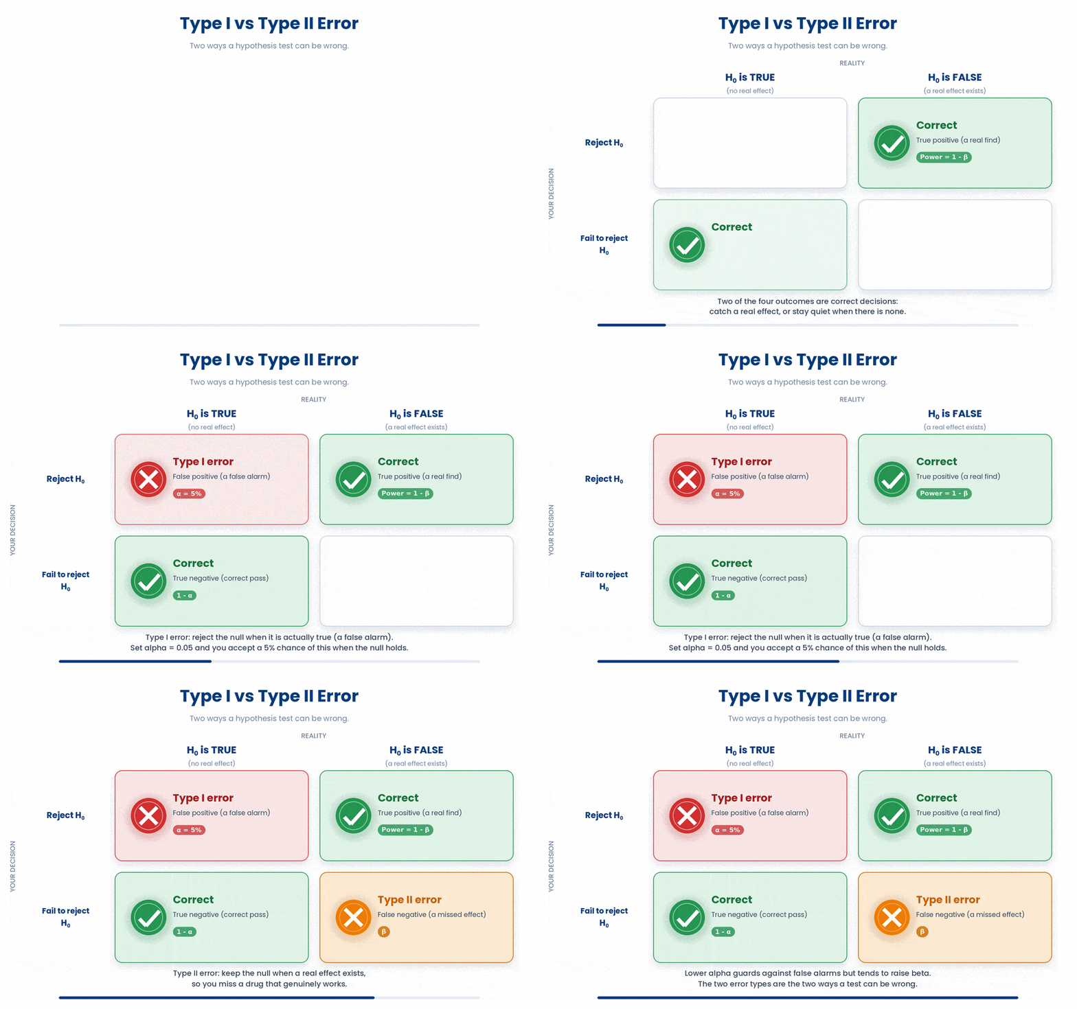
That false alarm is a Type I error: rejecting H0 when it is actually true — declaring an effect that is not there. Set alpha to 0.05 and you accept a 5% chance of this when the null holds. The opposite mistake is a Type II error: failing to reject H0 when there really is an effect — missing a drug that genuinely works.
The chance of a Type II error is called beta. Power is 1 - beta: the probability that your study detects a real effect of a given size. A study with 80% power has a 1-in-5 chance of missing a true effect. Power rises with the sample size, the effect size, and a looser alpha.
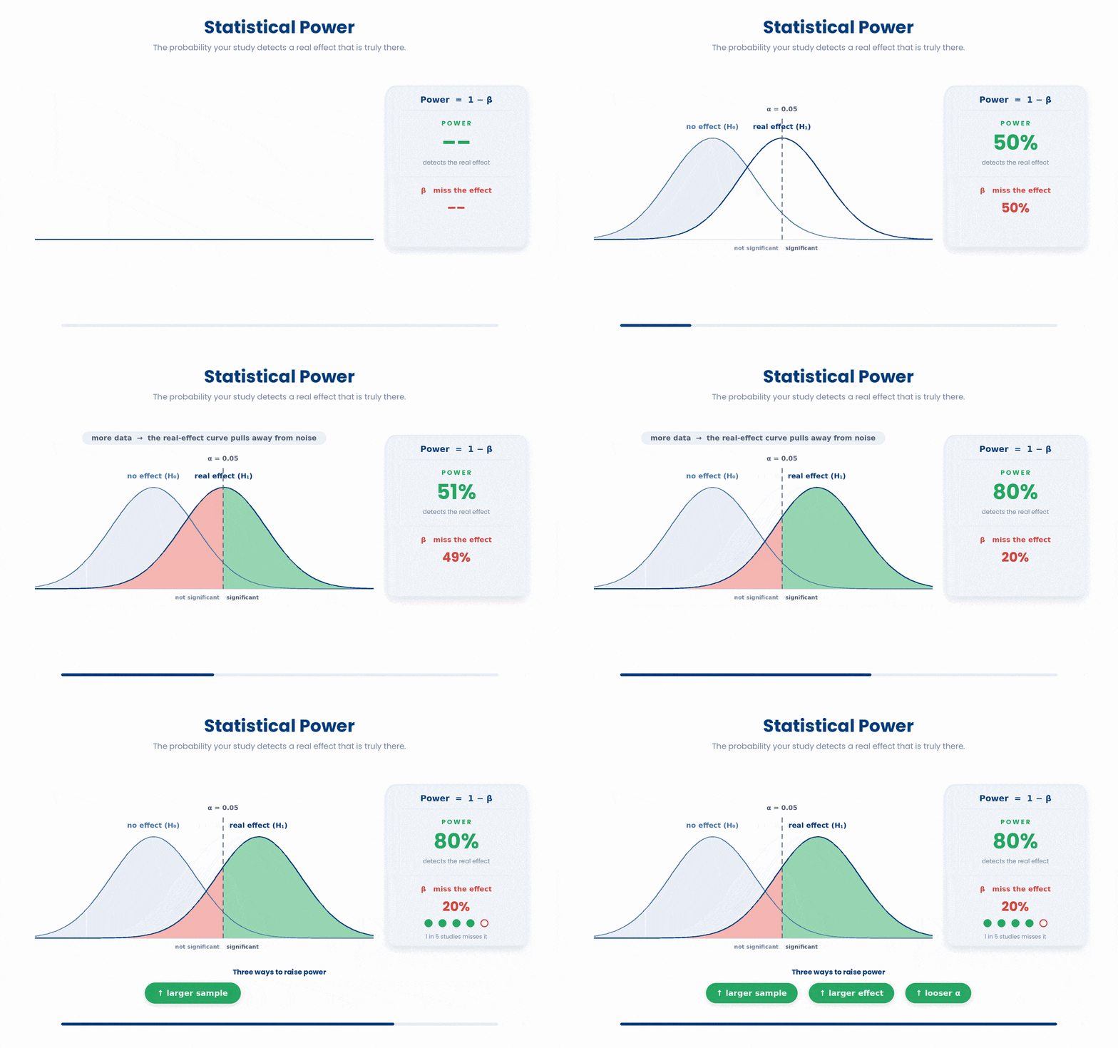
Here is the clinical danger. An underpowered study — too few patients — will miss real effects and return non-significant p-values even when the treatment works. A non-significant result from a tiny trial tells you almost nothing. This is why you plan sample size in advance.
3.1 Planning sample size with pwr
You can compute the sample size a study needs before running it. The pwr package ties together four quantities — effect size, sample size, alpha, and power. Give it any three and it solves for the fourth. For comparing two means, use pwr.t.test().
Suppose you want 80% power to detect a medium effect (Cohen's d of 0.5) at alpha 0.05, with equal-sized groups. Leave n out and pwr returns the n per group you need. Read the n in its printout.
Try this snippet in the R Scratchpad on the right.
library(pwr)
pwr.t.test(d = 0.5, sig.level = 0.05, power = 0.80, type = "two.sample")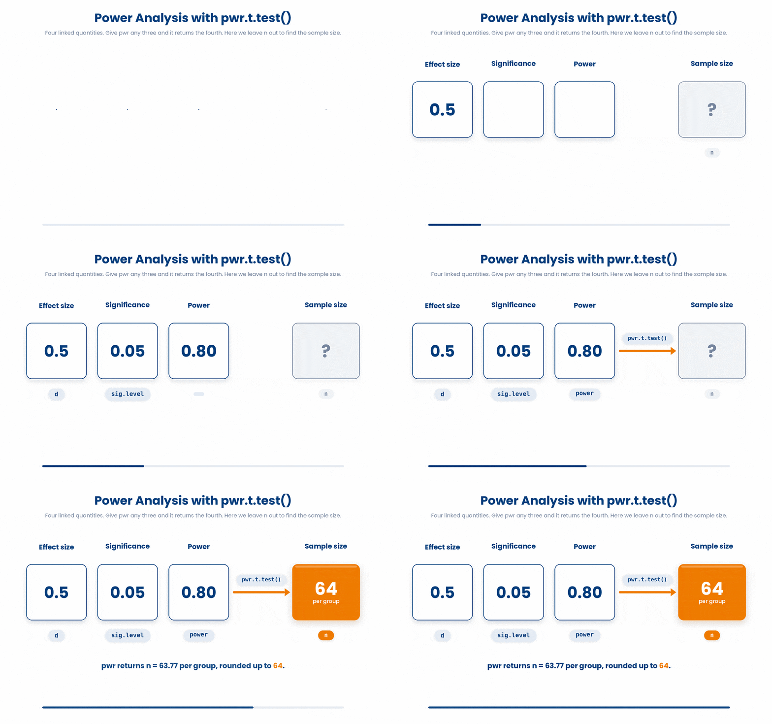
The novice habit to avoid: running the study first and computing power afterwards from the result you got. So-called post-hoc power adds nothing — it is just a rescaling of the p-value. Power analysis belongs at the planning stage, with an effect size you decide is clinically worth detecting.
4 One-sided vs two-sided, and statistical vs clinical significance
With alpha and power in hand, two final decisions shape how you report a test honestly: which direction you test in, and whether a significant result actually matters to a patient.
A two-sided test asks whether the groups differ at all — in either direction. A one-sided test asks only whether one group is greater than the other. A one-sided test has more power to detect an effect in the chosen direction, but it is blind to a difference the other way.
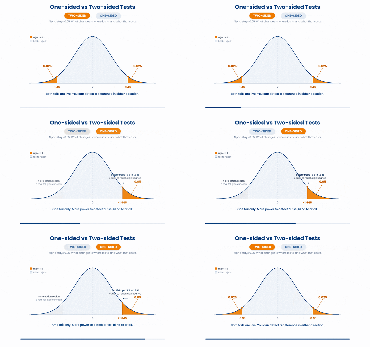
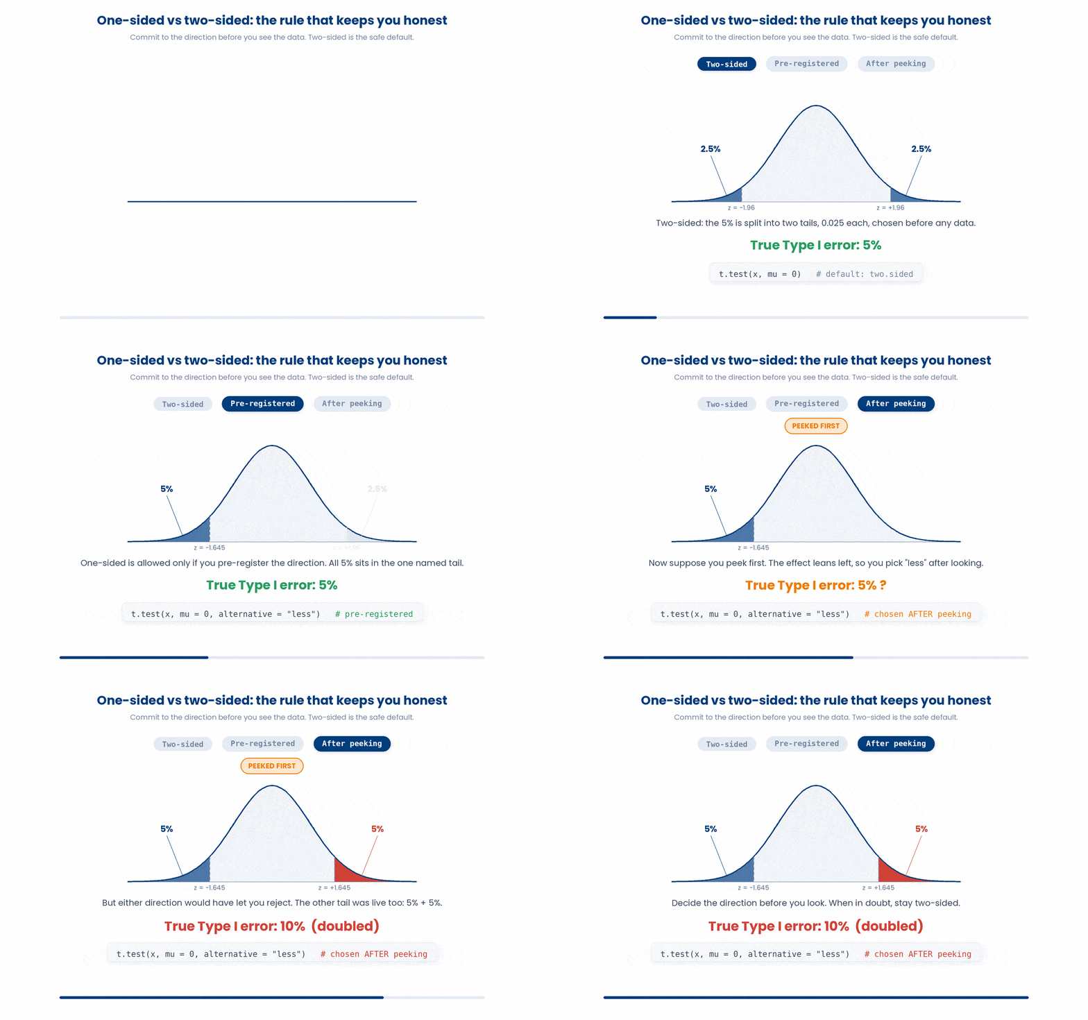
The rule that keeps you honest: commit to one-sided or two-sided BEFORE you see the data, and use two-sided as the safe default. Choosing one-sided after peeking — because the effect happened to point the way you hoped — quietly doubles your real Type I error. That is a form of cheating, even when unintentional.
In R the direction is the alternative argument to t.test(). The default is "two.sided"; you would write alternative = "less" only if you had pre-registered a one-directional hypothesis.
4.1 Statistical significance is not clinical significance
A result can be statistically significant — p below alpha — yet clinically meaningless. With ten thousand patients, a mean HbA1c difference of 0.02% can reach p < 0.001 while changing no treatment decision. Significance answers 'is it detectable?', not 'does it matter?'.
So report the effect, not just the verdict. Always report an effect estimate WITH a confidence interval in clinical units, not a bare p-value. 'HbA1c fell by 0.8% (95% CI 0.5 to 1.1)' tells a clinician how much and how precisely. 'p = 0.002' tells them almost nothing they can act on.

5 Choosing and running the right test
Everything so far has used a t-test, but the right test depends on your data: how many groups, what kind of outcome, and crucially whether the observations are paired. This section is your decision aid.
Match the question to the test by the shape of your data:
- t.test — compare a mean against a value (one-sample), or two group means (two-sample), or before-vs-after on the same patients (PAIRED).
- aov — compare the means of THREE or more groups at once (analysis of variance).
- wilcox.test / kruskal.test — the non-parametric alternatives when the outcome is skewed or ordinal, for two groups and for 3+ groups respectively.
- chisq.test / fisher.test / prop.test — for categorical data: an association in a table, or a comparison of proportions (fisher.test for small counts).
- cor.test — test whether two continuous measurements are correlated.
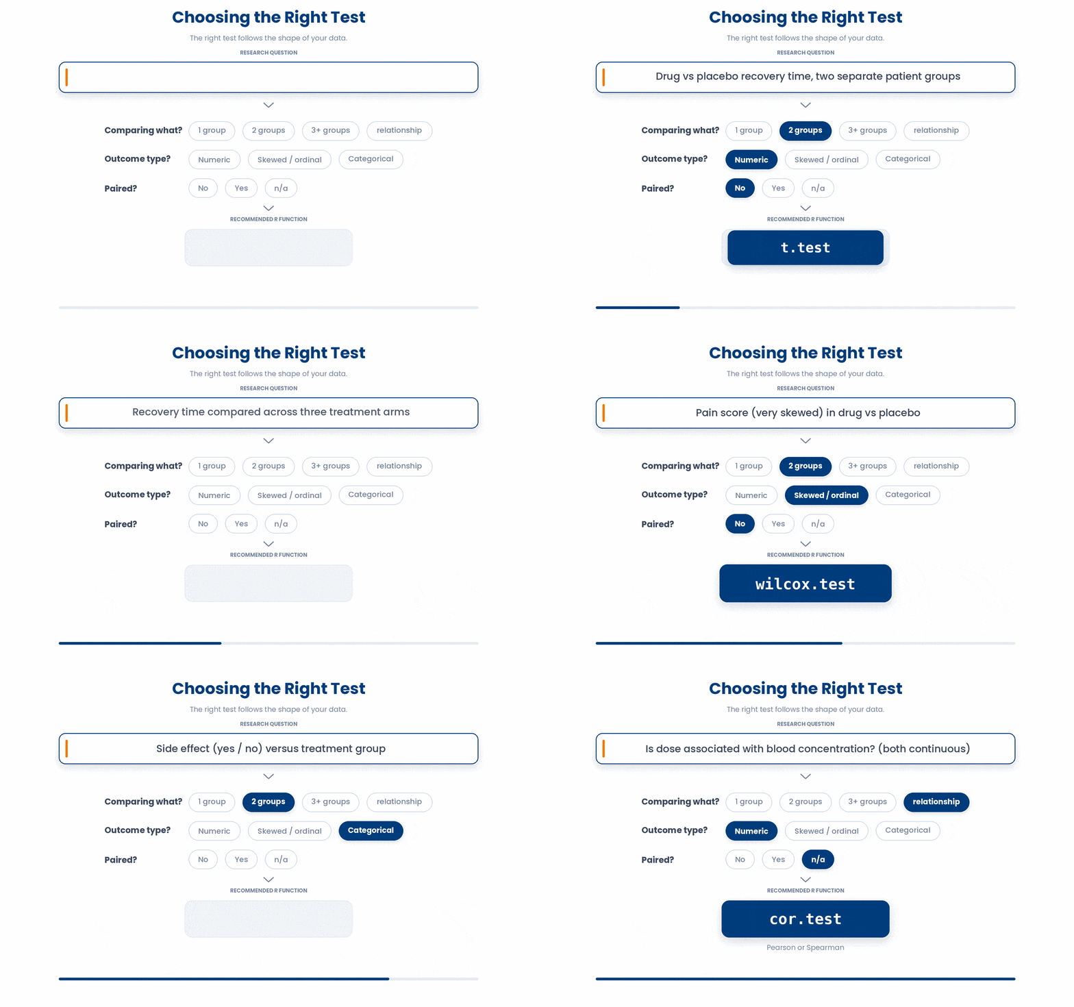
Each returns a tidy summary. Wrap any result in broom::tidy() to get a one-row tibble of the estimate, statistic, p-value, and CI — ideal for putting in a report or a table.
Try this snippet in the R Scratchpad on the right.
library(broom)
drug <- c(6.8, 7.1, 6.5, 7.4, 6.9)
placebo <- c(7.6, 8.0, 7.4, 7.9, 8.2)
tidy(t.test(drug, placebo))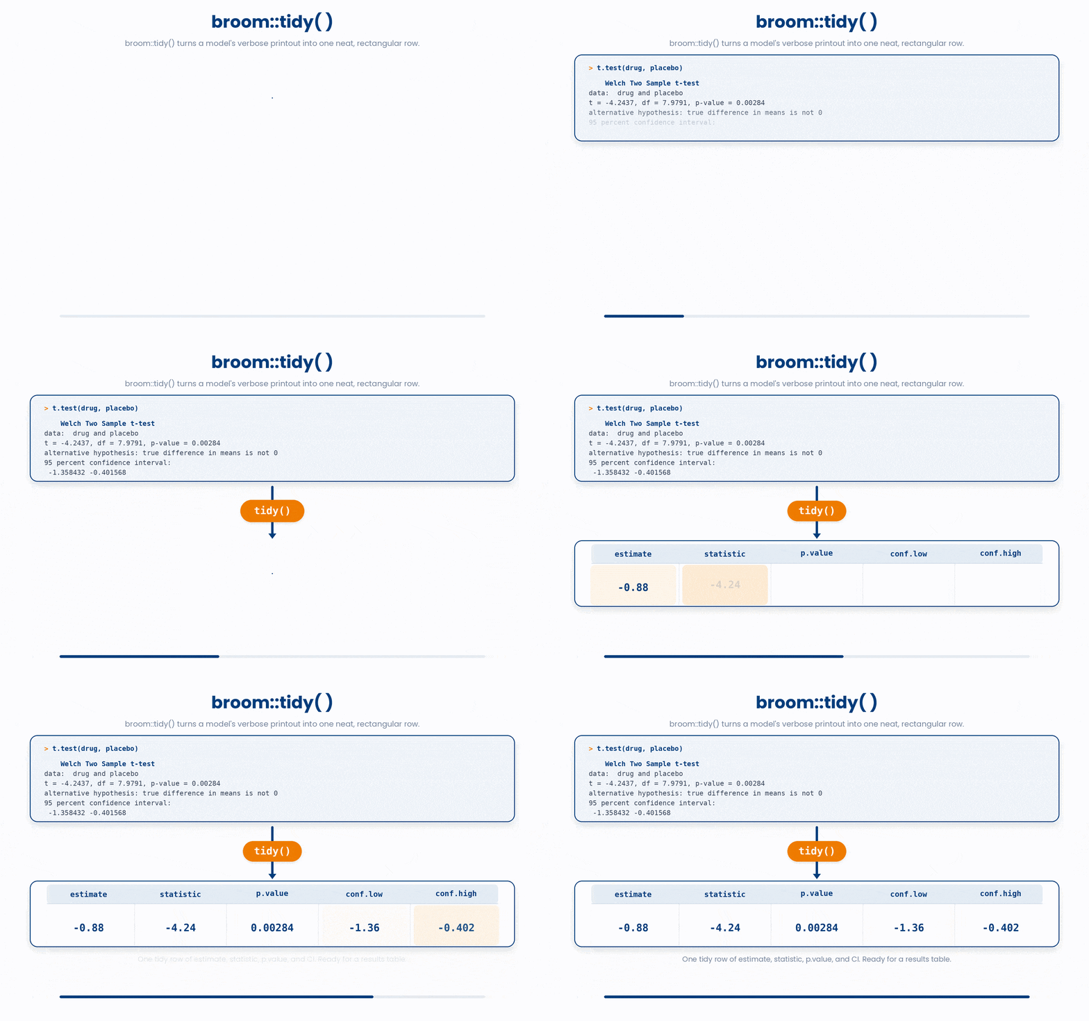
When the outcome is a category rather than a measurement, the test changes shape. Build a 2x2 of treatment arm against outcome and ask chisq.test() whether the two are associated.
Try this snippet in the R Scratchpad on the right.
tbl <- matrix(c(18, 12, 7, 23), nrow = 2, byrow = TRUE,
              dimnames = list(Arm = c("Drug", "Placebo"),
                              Outcome = c("Improved", "Not")))
tbl
chisq.test(tbl)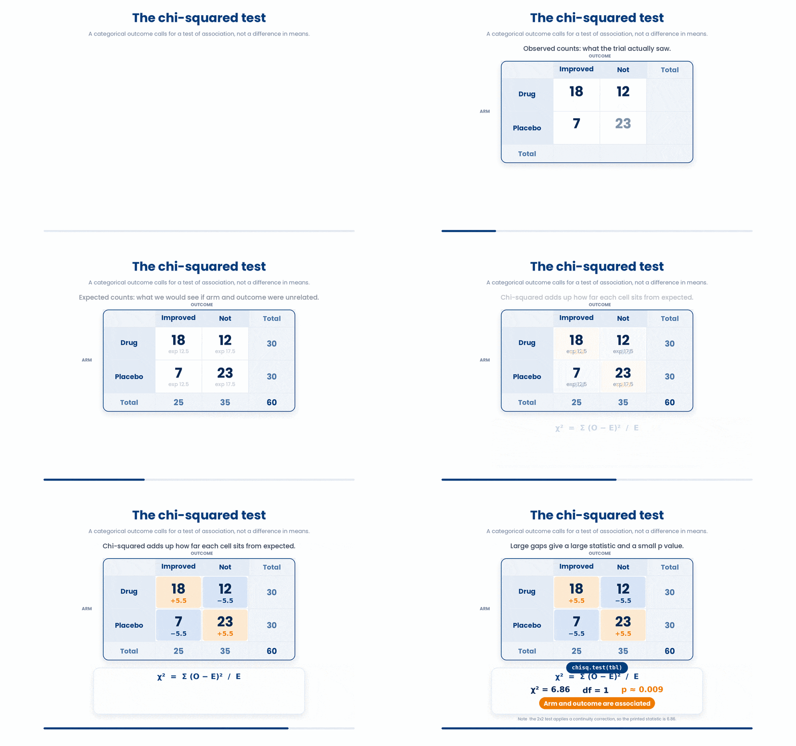
5.1 Paired data is the trap that catches everyone
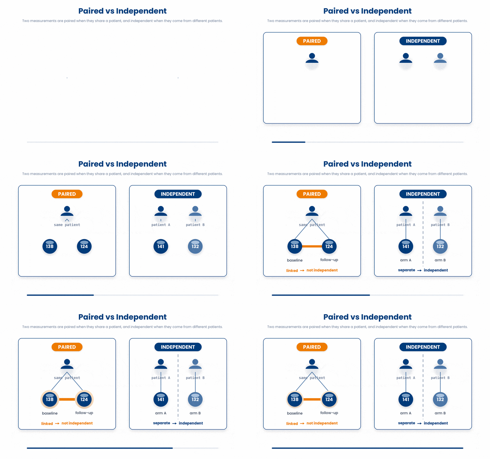
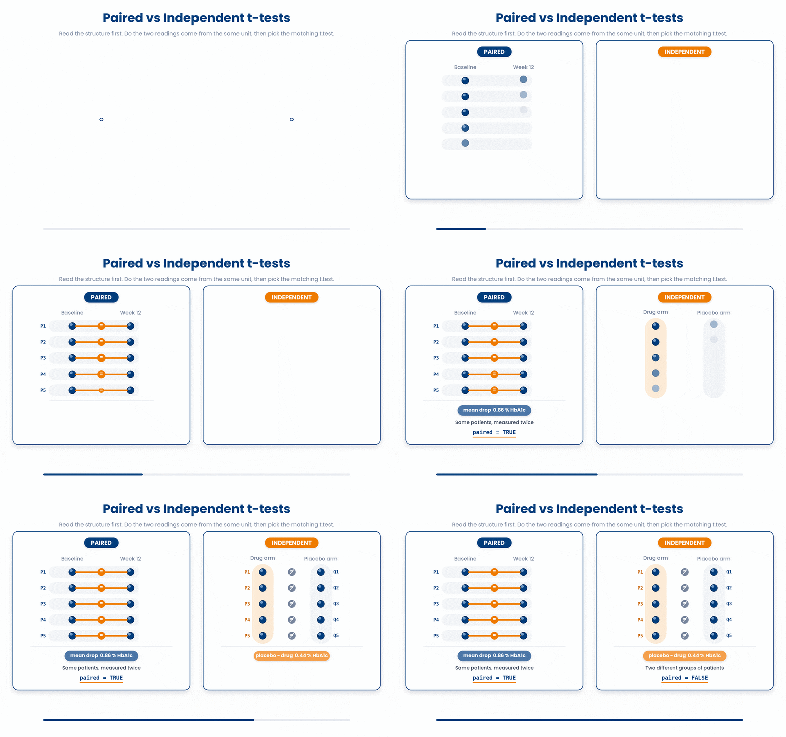
Two measurements are paired when they come from the same patient — a baseline and a follow-up, or a left eye and a right eye. They are linked, so they are not independent. Data are independent instead when each value comes from a different patient, as in two separate treatment arms.
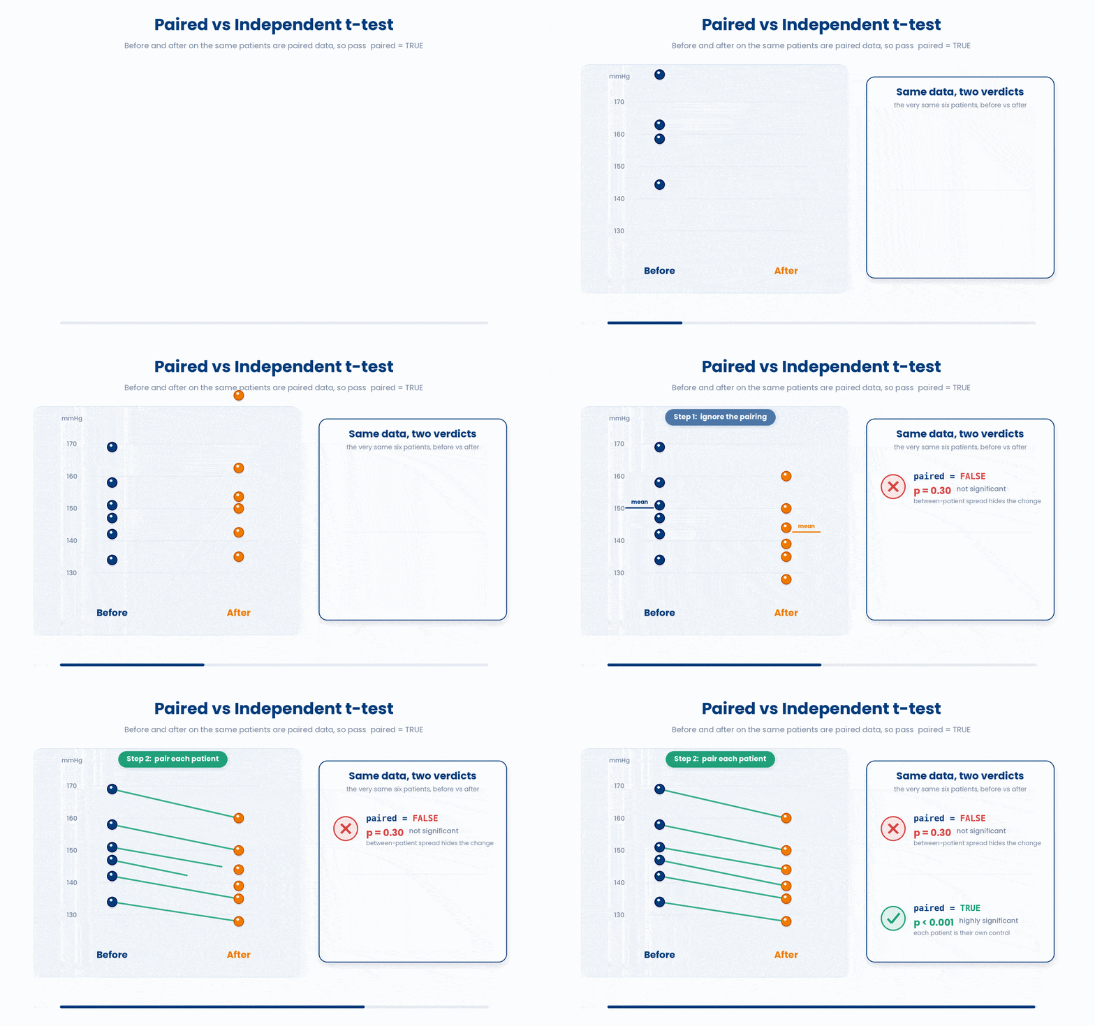
Here is the single most common test-selection error: running an independent-samples test on paired data. For before-vs-after on the same patients, you must pass paired = TRUE to t.test(). A paired test compares each patient to themselves, removing between-patient variation, so it is far more powerful — and ignoring the pairing gives a wrong p-value.
Watch for the same structure under other names: repeated measures over time, and clustered data such as several samples from one patient or several patients from one ward. Whenever observations share a source, they are not independent, and a plain two-sample test is wrong.
Try this snippet in the R Scratchpad on the right.
baseline <- c(8.1, 7.8, 9.0, 8.4, 7.9)
followup <- c(7.2, 7.0, 8.1, 7.5, 7.1)
t.test(baseline, followup, paired = TRUE)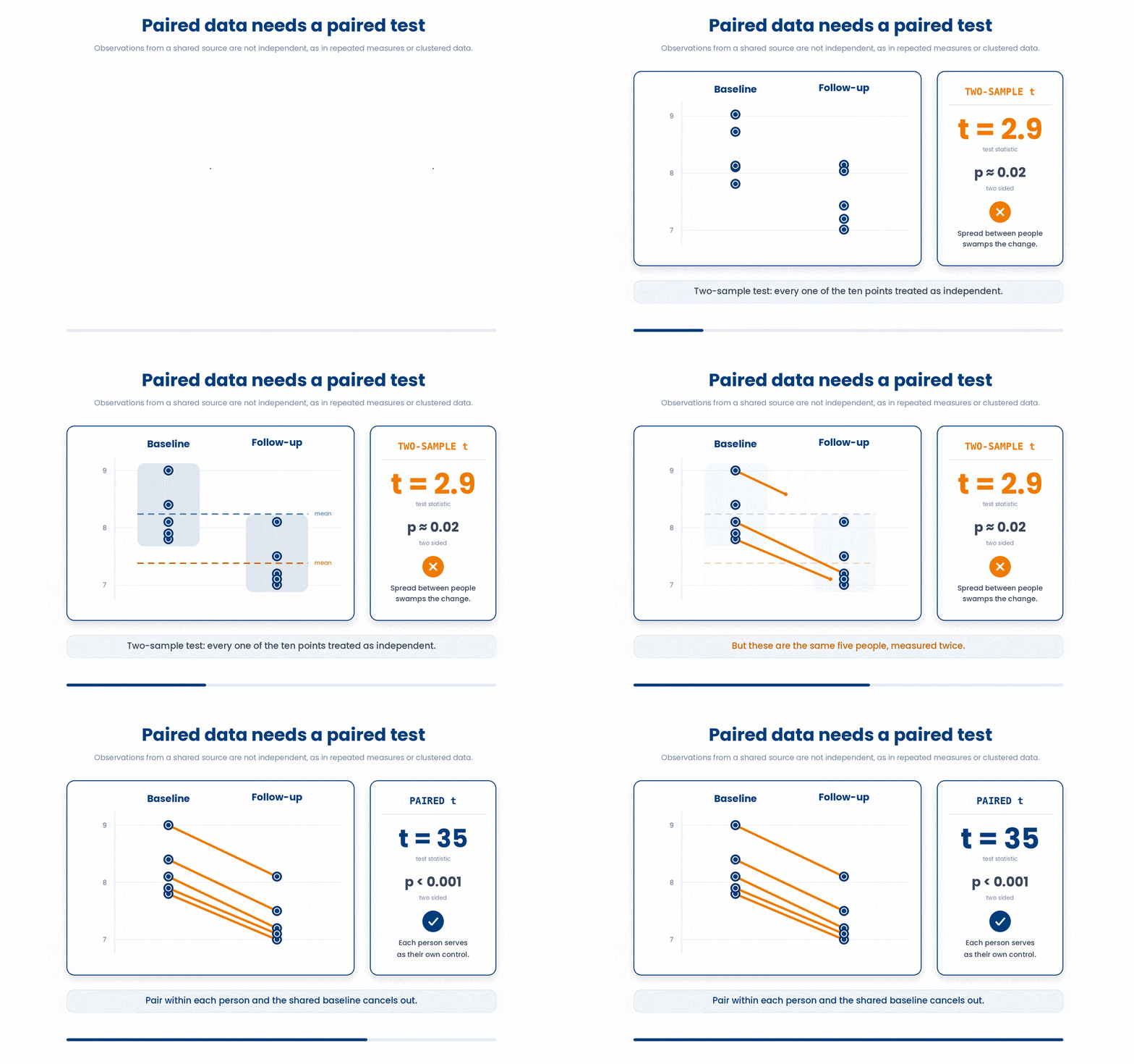
5.2 Check the assumptions first
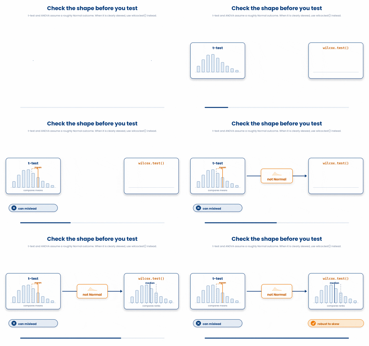
A t-test and ANOVA assume the outcome is roughly Normal and the observations are independent. Running a t-test on a skewed or ordinal outcome without checking can mislead you — switch to wilcox.test() when the data are clearly non-Normal.
Check approximate Normality two ways. A QQ plot plots your data against what a Normal distribution would predict; points near the straight line mean roughly Normal. The Shapiro-Wilk test (shapiro.test()) gives a formal p-value, where a small p flags non-Normality. Use the plot as your main guide; the test alone over-flags in large samples.
Draw a QQ plot for a small sample of lab values. A base-R plot appears as soon as you call the plotting function — no printing needed.
Try this snippet in the R Scratchpad on the right.
hba1c <- c(7.2, 8.1, 6.5, 9.4, 7.0, 8.8, 6.9, 7.6)
qqnorm(hba1c)
qqline(hba1c)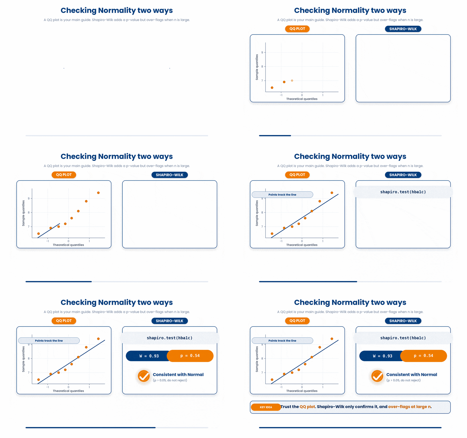
When the QQ plot bends away from the line, switch to the non-parametric wilcox.test() — it compares ranks, not means, so a skewed outcome cannot distort it.
Try this snippet in the R Scratchpad on the right.
drug <- c(6.8, 7.1, 6.5, 7.4, 6.9)
placebo <- c(7.6, 8.0, 7.4, 7.9, 8.2)
wilcox.test(drug, placebo)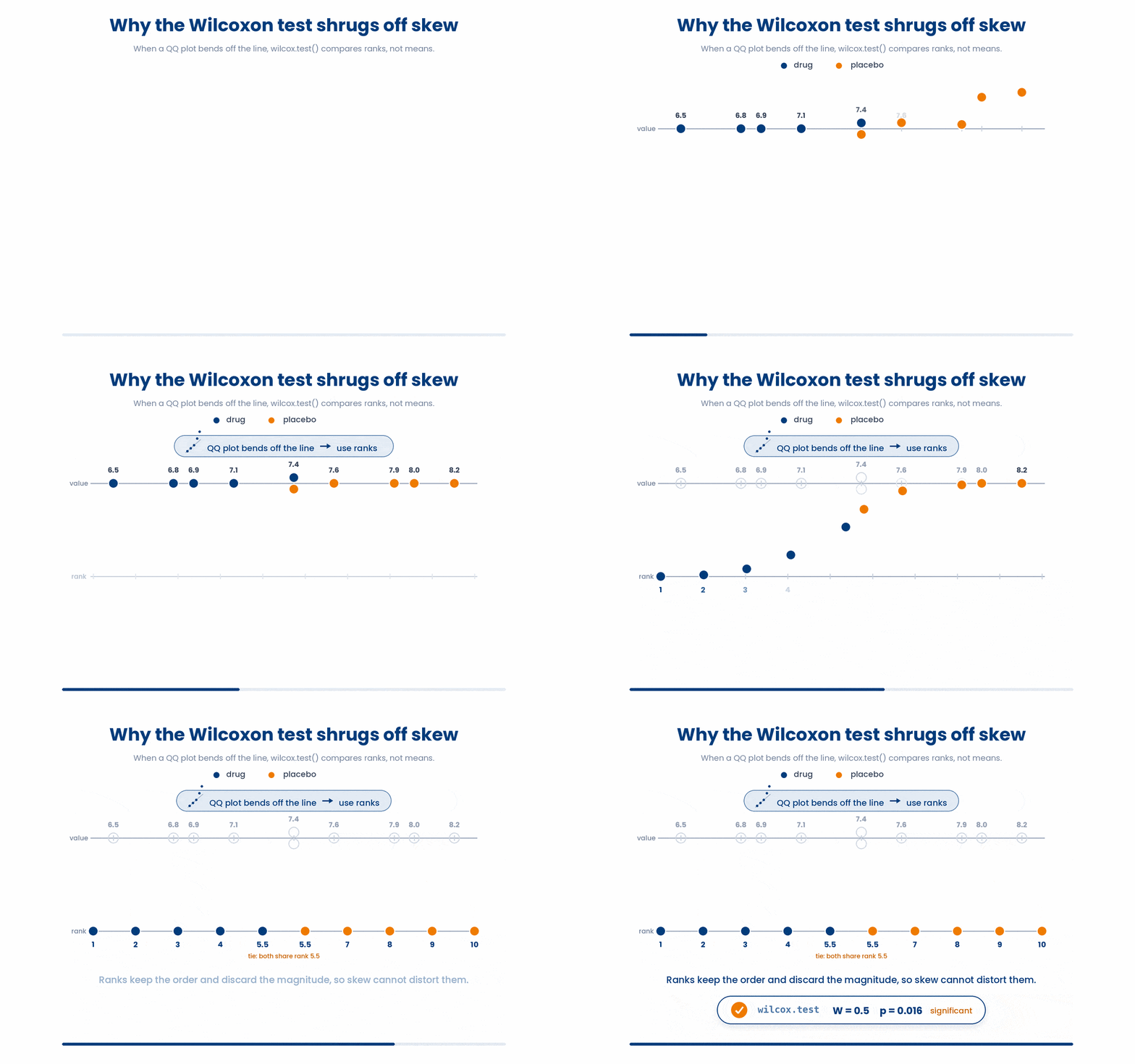
6 Put it together
This Parsons problem gives you the right lines in the wrong order, plus a few lines that do not belong. Drag the correct lines into order and leave the wrong ones in the bank.
All the lines you need are in the Line bank on the left — some may be distractors you should leave behind. Drag the lines you need into the Your solution column on the right, in the correct order, then click Check.
Task: Switch on broom, store each patient's baseline and follow-up HbA1c, run a PAIRED t-test because the readings come from the same patients, then tidy it into a one-row table.
tidy(chisq.test(baseline, followup))library(broom)tidy(t.test(baseline, followup, paired = FALSE))baseline <- c(8.1, 7.8, 9.0, 8.4, 7.9)followup <- c(7.2, 7.0, 8.1, 7.5, 7.1)library(paired)tidy(t.test(baseline, followup, paired = TRUE))
- Drop lines here, in order.
Now you will make the call that trips up most beginners: spotting which comparison in a trial is PAIRED and which is INDEPENDENT, then running each with the right test and reporting the effect in clinical units. The worked example fades its support — study the full solution, then fill the gap, then solve a fresh one.
Work through this example in three stages. You unlock each stage only after the tutor confirms the previous one. Each stage removes more of the scaffolding — by the end you are writing it yourself.
Problem: Five patients on a new drug have HbA1c measured at baseline and after 12 weeks. The baseline-vs-followup comparison is WITHIN the same patients, so it is paired: use a paired t-test. Run it, then report the mean drop in HbA1c (clinical units).
baseline <- c(8.1, 7.8, 9.0, 8.4, 7.9)
followup <- c(7.2, 7.0, 8.1, 7.5, 7.1)
t.test(baseline, followup, paired = TRUE)
round(mean(baseline) - mean(followup), 2)- The two readings come from the SAME patients, so the comparison is paired
- Pass paired = TRUE to t.test so it compares each patient to themselves
- Report the effect in clinical units: the mean fall in HbA1c, here mean(baseline) - mean(followup)
The same solution with key parts replaced by ???.
Fill in every ??? so the code matches the reference,
then ask the tutor to check it.
Your turn: Now compare the 12-week HbA1c of the drug arm (the followup values above) against a SEPARATE placebo arm of five different patients with values 7.6, 8.0, 7.4, 7.9, 8.2. These are different patients, so the comparison is INDEPENDENT: use a two-sample t.test (no paired = TRUE). Report the mean difference, placebo minus drug, in clinical units.
7 Check your understanding
You have reached the end of the module. Try the same questions again — your answers here, paired with your pre-test answers, are how we measure what the module taught you. Answer every question and confidence rating, then click Submit and see results to view your score.
You set alpha = 0.05 and your test returns p = 0.02. What does alpha represent here?
A regulator rejects a drug's null hypothesis of no effect, but in truth the drug does nothing. Which error is this?
A trial is designed with 80% power to detect a clinically important effect. What does this mean?
An underpowered trial of 8 patients returns a non-significant p-value for a drug that truly works. What most likely happened?
You want the n per group for 80% power to detect Cohen's d of 0.5 at alpha 0.05. Which call solves for it?
You decide to switch to a one-sided test only after seeing the effect points the way you hoped. Why is this a problem?
With 10,000 patients, a mean HbA1c difference of 0.02% reaches p < 0.001. How should you report it?
You compare a continuous, roughly Normal outcome across THREE treatment arms at once. Which test fits?
I can explain alpha, Type I and Type II error, and power in plain clinical words, and say why an underpowered study can miss a real effect.
I can plan a study's sample size with pwr.t.test(), commit to a one-sided or two-sided test before seeing the data, and tell statistical significance from clinical significance.
I can recognise whether data are paired or independent, choose and run the correct base-R test after checking its assumptions, and tidy the result with broom::tidy().
8 Your results
Here is how your post-test answers compare with your pre-test answers. The pre/post pairing is the most reliable way to see what this module actually taught you.
Submit the post-test to see your results.
What is the one thing from this module that is still unclear to you?