

1 Before you start
This is not graded, and it does not count towards anything. Answer every question even if you are only guessing — having a go at something before you have been taught it is one of the best ways to remember it afterwards. The lesson ends with another short check, and there you will be shown the correct answer for anything you missed. Choose an option for every question and confidence rating, then click Submit answers.
You have eight HbA1c readings in a vector and want a 95% confidence interval for the mean. Which line gives it to you directly?
A rough 95% confidence interval for a mean is the estimate give or take about how many standard errors?
Why does t.test() give a slightly wider interval than the by-hand estimate mean(x) + c(-1.96, 1.96) * se for a small sample?
A study reports mean HbA1c 7.8, 95% CI [7.2, 8.4]. Which statement is the correct interpretation of the 95%?
In a clinic, 38 of 200 patients reached their HbA1c target. Which call returns a 95% confidence interval for that proportion?
You have only 4 events out of 30 patients and want a confidence interval for the proportion. Which function is the safer choice for such small counts?
Length of stay is strongly right-skewed and you want a 95% confidence interval for its median. Which approach fits?
You built a bootstrap distribution of medians in boot_meds. Which line reads off the 95% confidence interval?
I can build a 95% confidence interval for a mean in R with t.test(), read it off with $conf.int, and state correctly that the 95% refers to the procedure across many studies rather than the one interval.
I can build a confidence interval for a proportion with prop.test() or the exact binom.test(), and choose binom.test() when the event count is small.
I can bootstrap a 95% confidence interval for a skewed median with sample(replace = TRUE), replicate(), and quantile(), and report any estimate as "estimate, 95% CI [low, high]".
2 Introduction
In Part I you saw the Central Limit Theorem make the sample mean bell-shaped, and you learned that the standard error measures how much that mean would wobble if you ran the study again. This part cashes that in: it turns a single estimate into a confidence interval — a stated range of plausible values for the population truth you could not measure directly.
This part of the module covers five skills — building each interval in R, plus reading what it means and reporting it cleanly:
- A confidence interval for a mean — build it once by hand as the estimate give or take 1.96 standard errors, then let t.test() do it properly, and read the range off with $conf.int.
- What the 95% really means — a property of the procedure across many repeated studies, not a probability for the one interval on your screen.
- Intervals for a proportion — a large-sample interval with prop.test() and the exact binom.test() you reach for when the event count is small.
- A skewed median by bootstrap — resample your own data with sample(x, replace = TRUE), recompute the median many times, and read the middle 95% off with quantile() — no formula required.
- Reporting the result — in one consistent shape, "estimate, 95% CI [low, high]", pulling the numbers cleanly with broom::tidy() rather than copying them by hand.
By the end of this part you will be able to build a 95% confidence interval for a mean, a proportion, and a skewed median in R, state correctly what the 95% refers to, and report any estimate as "estimate, 95% CI [low, high]".
Try every snippet in the R Scratchpad on the right. The dataset diabetes_clinic.csv is already loaded, and the small vectors and bootstrap simulations build their own data with c(), set.seed(), and replicate(), so you can run everything as you read.
3 A 95% confidence interval for a mean
The CLT lets us go from a point estimate to a range. A confidence interval is a range of plausible values for the population parameter, built from your sample so that the procedure traps the true value 95% of the time. For a mean, R hands you the whole interval through t.test().
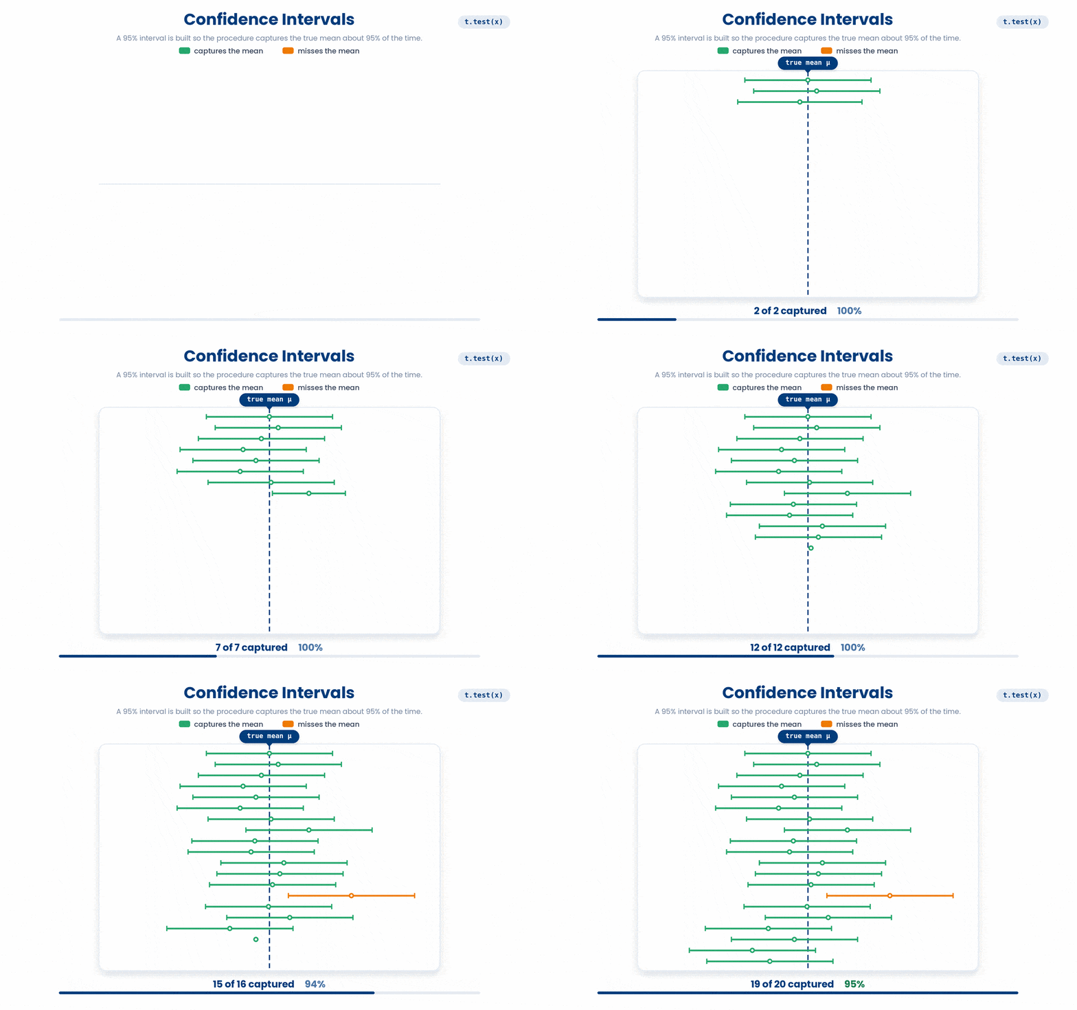
You already have the pieces. A rough 95% interval is the estimate give or take about 1.96 standard errors — that 1.96 is the qnorm(0.975) cut-off from the Normal curve in Part I. Build it by hand once, then let t.test() do it properly (it uses the slightly wider t-distribution for small samples).
Try this snippet in the R Scratchpad on the right.
hba1c <- c(7.2, 8.1, 6.5, 9.4, 7.8, 6.9, 8.4, 7.1)
se <- sd(hba1c) / sqrt(length(hba1c))
mean(hba1c) + c(-1.96, 1.96) * se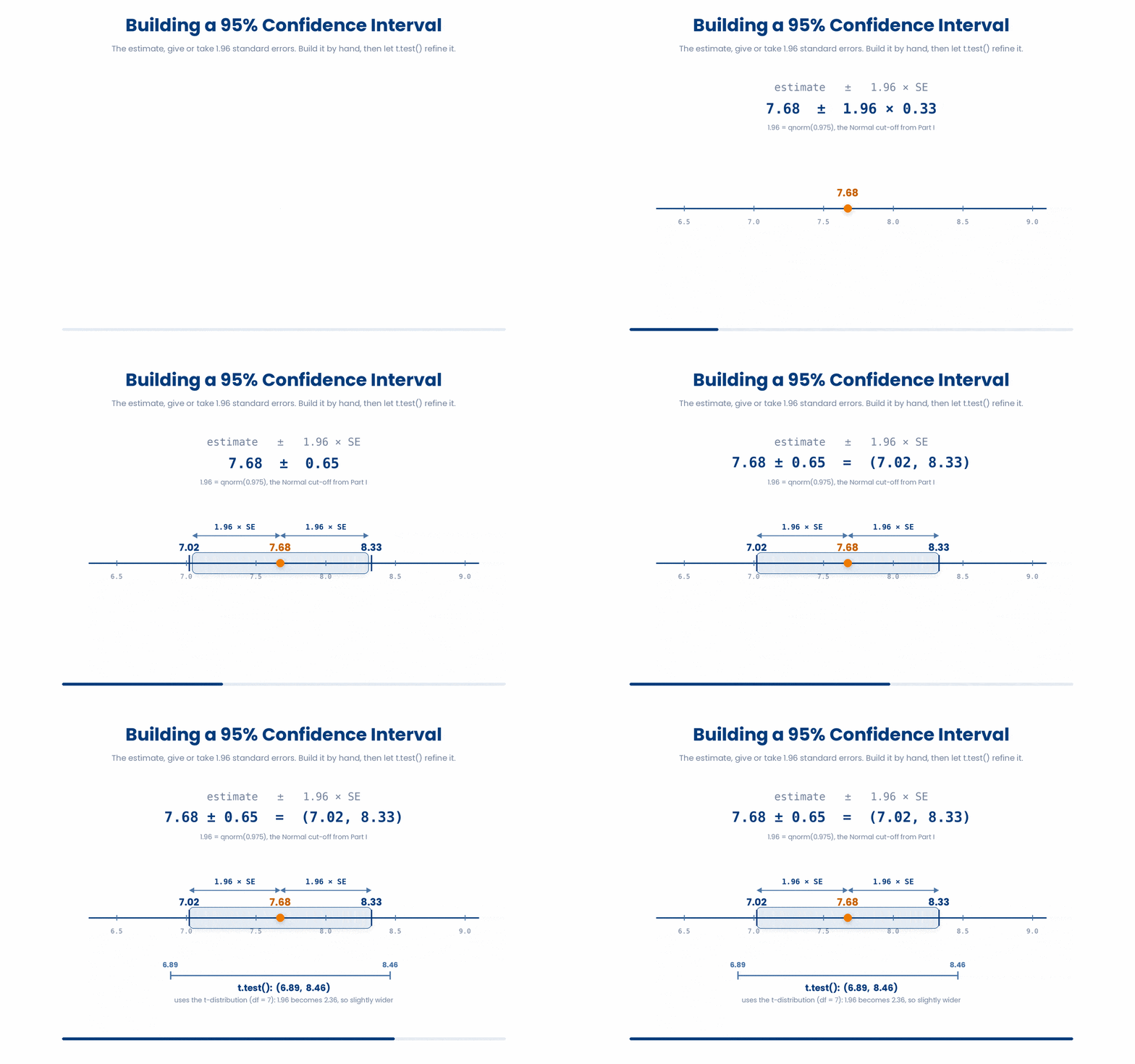
You do not need the t-distribution algebra. Call t.test on your vector and read the confidence interval off the result, or pull it out cleanly with $conf.int.
Try this snippet in the R Scratchpad on the right.
hba1c <- c(7.2, 8.1, 6.5, 9.4, 7.8, 6.9, 8.4, 7.1)
t.test(hba1c)
t.test(hba1c)$conf.int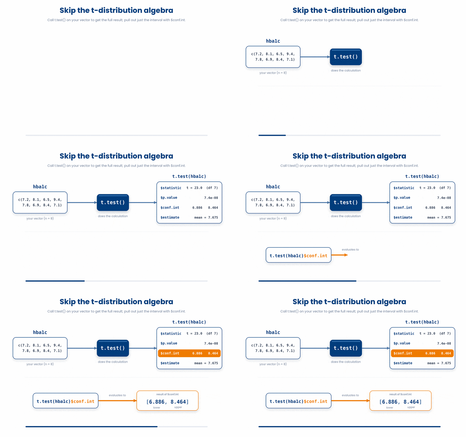
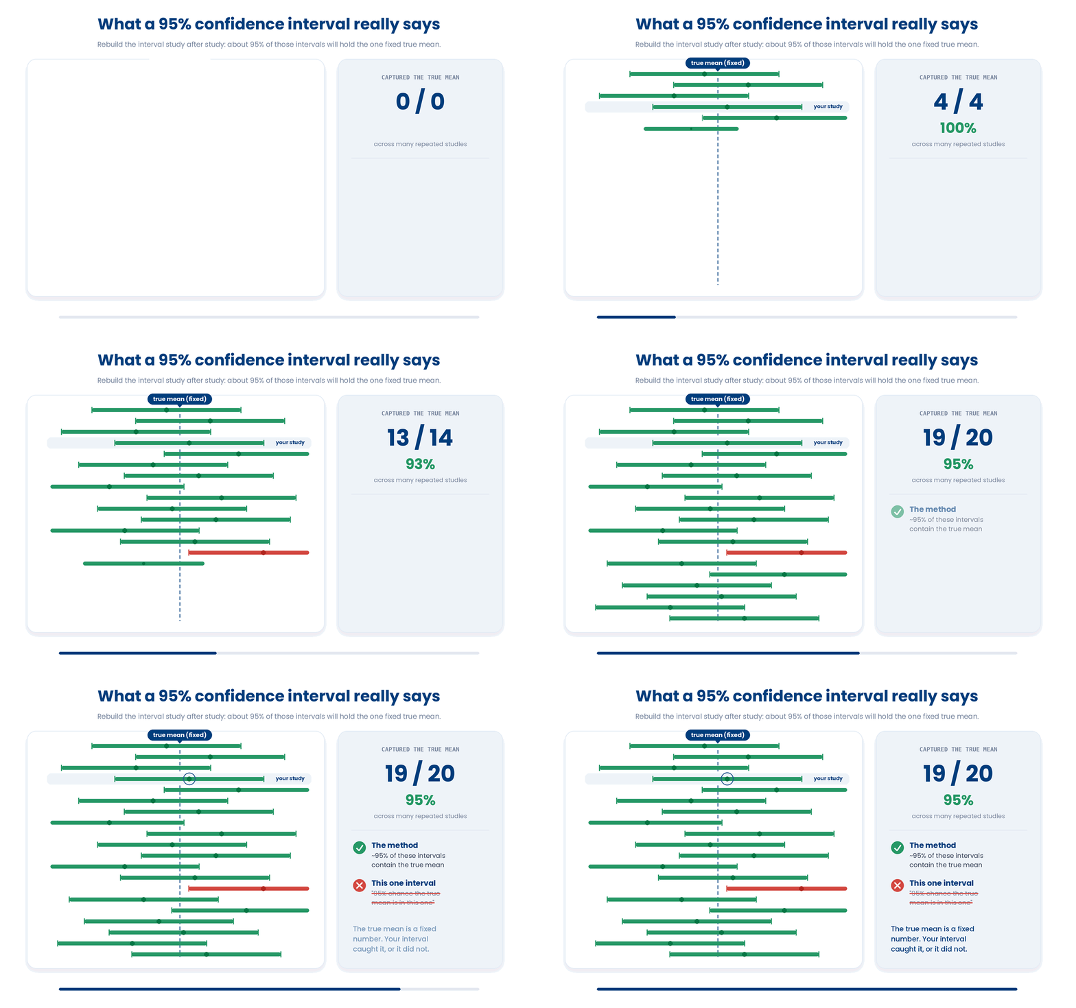
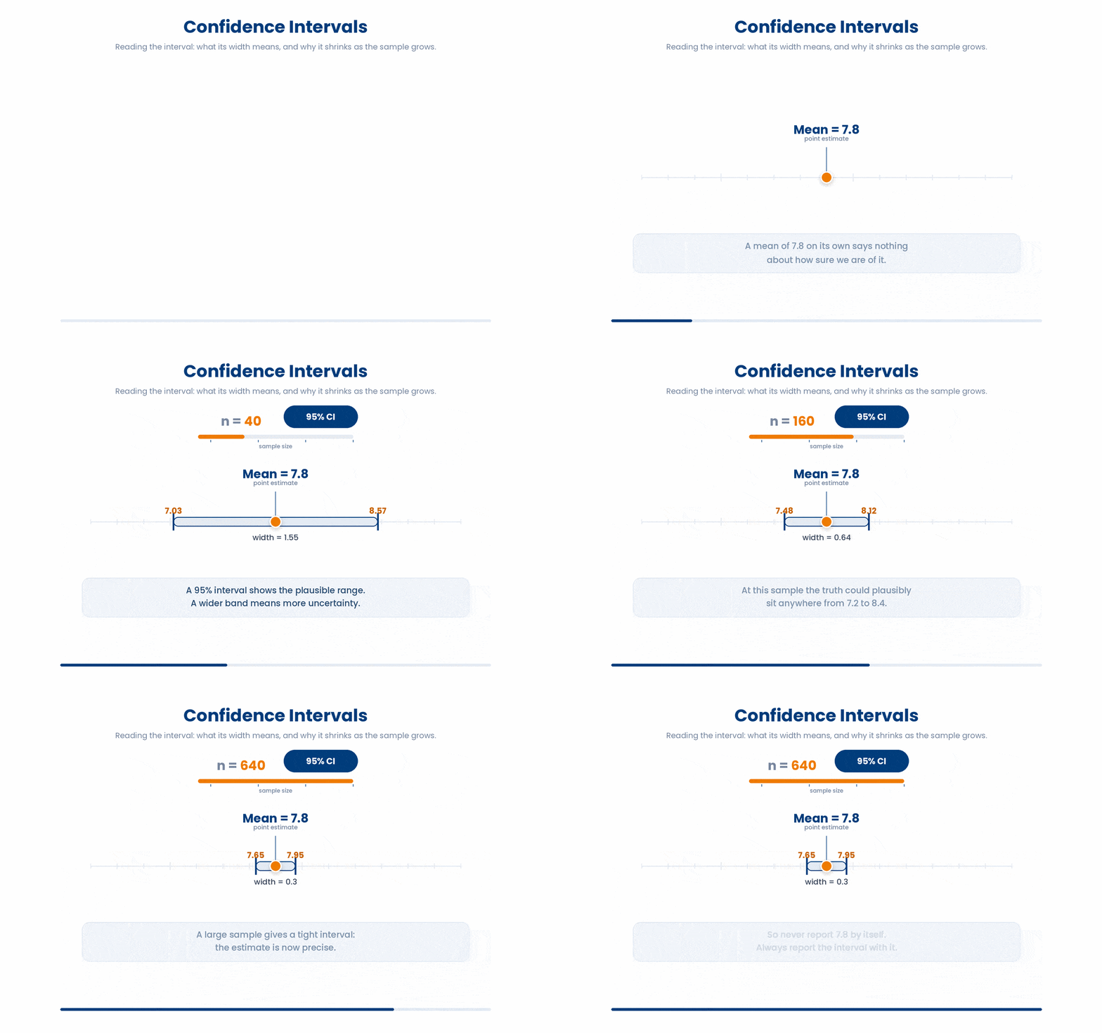
Now the interpretation that examiners and reviewers care about most. The 95% describes the long-run behaviour of the procedure, not a probability for this one interval. If you repeated the whole study many times and built an interval each time, about 95% of those intervals would contain the true mean.
Say it the wrong way and you have made the most famous error in statistics. It is wrong to say "there is a 95% probability the true mean lies in this interval." The true mean is a fixed number; your specific interval either caught it or did not. The 95% is a property of the method across many studies, not of the single interval on your screen.
A wider interval means more uncertainty. Intervals shrink as the sample grows, for the same square-root reason the SE shrinks. And never report a bare point estimate with no interval — a mean of 7.8 alone hides whether the truth could plausibly be 7.2 or 8.4, which changes the clinical story entirely.
4 Intervals for a proportion and for a skewed median
Means are not the only estimates that need an interval. Proportions and medians do too, and R has a clean function for each. This section finishes your toolkit.
4.1 A proportion with prop.test() or binom.test()
Suppose 38 of 200 patients reached their HbA1c target. The sample proportion is 0.19, but you owe the reader an interval. prop.test gives a large-sample interval; binom.test gives an exact one, which you prefer when counts are small.
Try this snippet in the R Scratchpad on the right.
prop.test(38, 200)
binom.test(38, 200)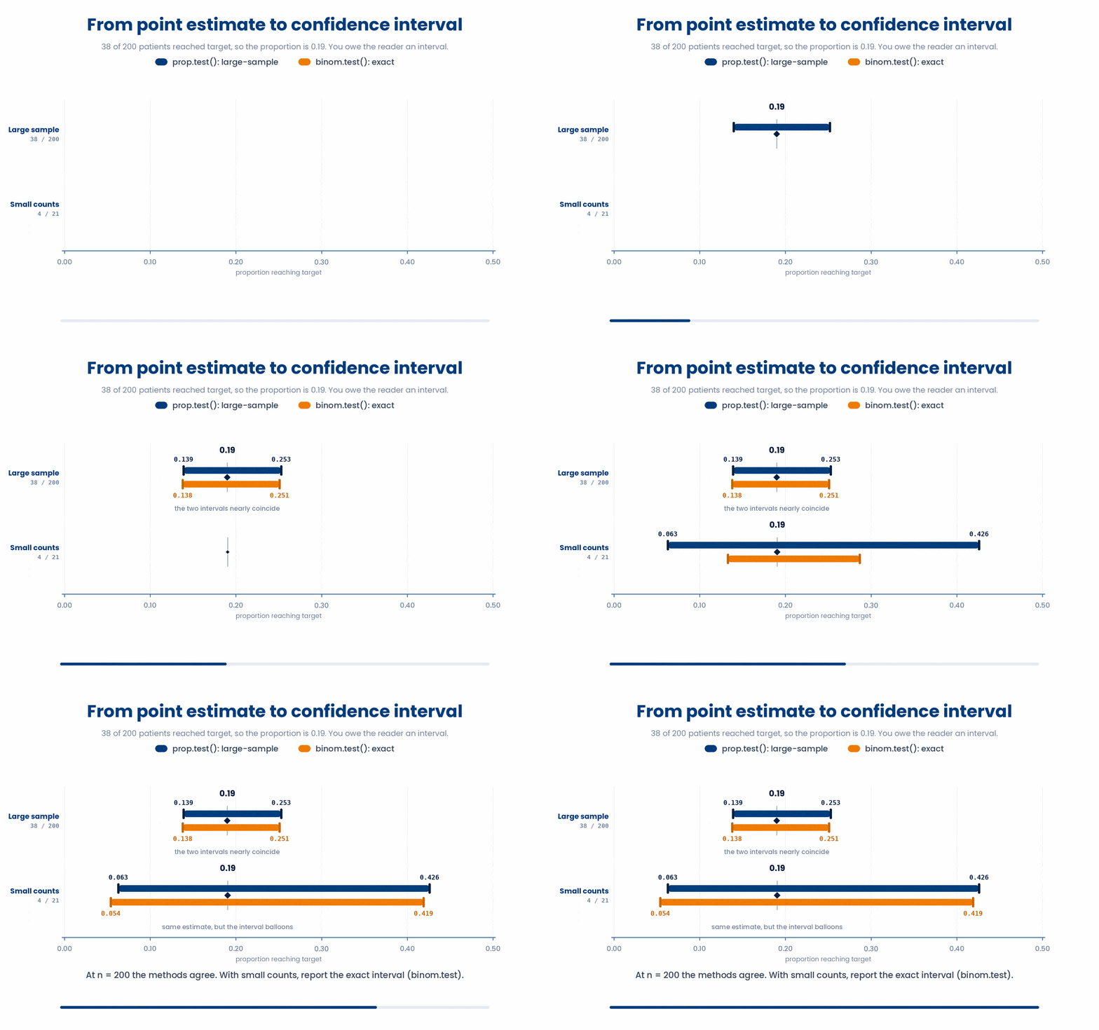
Read the interval the same procedural way as the mean: the method, repeated across many studies, would trap the true proportion 95% of the time. Reach for the exact binom.test() when you have only a handful of events, where the large-sample approximation gets shaky.
4.2 A skewed median by bootstrap
What if you want an interval for a median from skewed data, where no neat formula applies? You bootstrap it: resample your own data with replacement many times, recompute the median each time, and read the middle 95% of those medians as your interval.
IMAGE GIF_bootstrap_median
A median's confidence interval can be read straight off your own data by resampling it with replacement many times and keeping the middle 95% of the resulting medians, no formula required.
The building blocks are familiar. sample(x, replace = TRUE) draws a resample the same size as x; replicate() repeats it; quantile with c(0.025, 0.975) cuts off the lowest and highest 2.5% to leave the central 95%.
Try this snippet in the R Scratchpad on the right.
set.seed(2025)
los <- rexp(120, rate = 1 / 5)
boot_meds <- replicate(2000, median(sample(los, replace = TRUE)))
quantile(boot_meds, c(0.025, 0.975))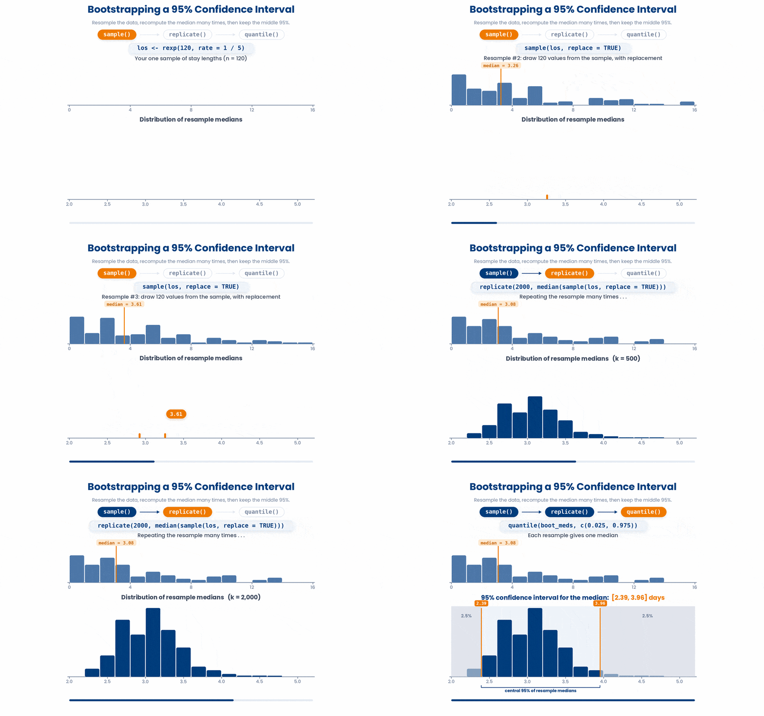
The two numbers you get back are the lower and upper limits of a 95% bootstrap confidence interval for the median. The same set.seed() habit applies — fix it so the interval is reproducible.
4.3 Report it: estimate, 95% CI [low, high]
However you got the interval, report it in one consistent shape: the point estimate, then "95% CI", then the low and high in square brackets — for example, "mean HbA1c 7.8, 95% CI [7.2, 8.4]". The estimate tells the reader your best guess; the interval tells them how sure to be.
![A reported result pairs one best-guess value with an interval of plausible values around it, and the convention is to write them in a fixed order: the estimate, then 95% CI, then [low, high].](GIF_ci_reporting.gif)
Pull the numbers programmatically rather than copying by hand. tidy from the broom package turns any t.test() or prop.test() result into a tidy one-row table with estimate, conf.low, and conf.high columns you can read or drop straight into a report.
Try this snippet in the R Scratchpad on the right.
library(broom)
hba1c <- c(7.2, 8.1, 6.5, 9.4, 7.8, 6.9, 8.4, 7.1)
tidy(t.test(hba1c))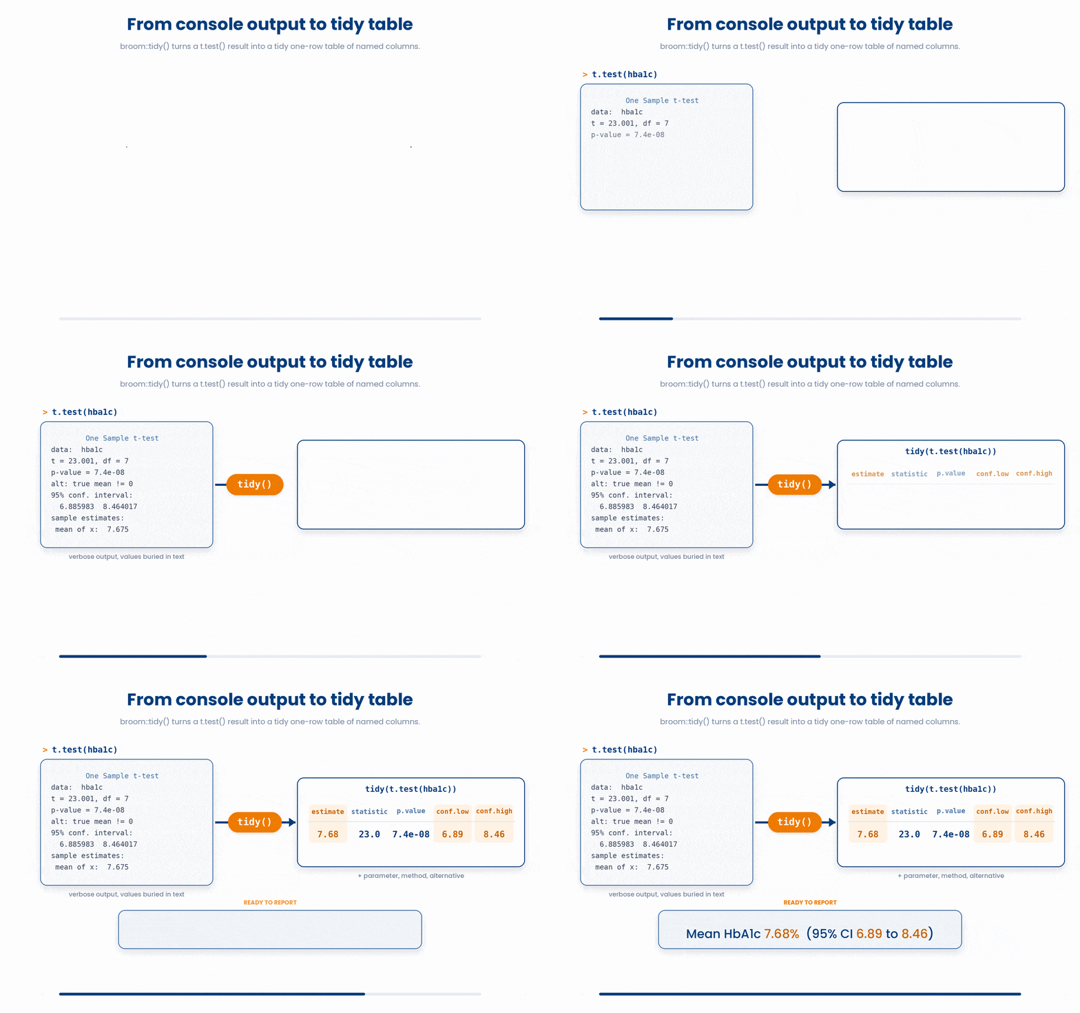
5 Put it together
The worked example below fades its support: first study a full solution, then fill the gap, then solve a fresh one on your own. It estimates a mean with a t.test interval and recomputes the standard error by hand.
Work through this example in three stages. You unlock each stage only after the tutor confirms the previous one. Each stage removes more of the scaffolding — by the end you are writing it yourself.
Problem: A small cohort had these systolic blood pressures (mmHg): 132, 145, 128, 151, 139, 136. Report the mean with its 95% confidence interval, then recompute the standard error of the mean by hand.
sbp <- c(132, 145, 128, 151, 139, 136)
t.test(sbp)$conf.int
sd(sbp) / sqrt(length(sbp))- Store the six readings in a vector with c()
- t.test(sbp)$conf.int gives the 95% confidence interval for the mean
- the standard error is the SD divided by the square root of the sample size, sd(sbp) / sqrt(length(sbp))
The same solution with key parts replaced by ???.
Fill in every ??? so the code matches the reference,
then ask the tutor to check it.
Your turn: Now do the same for four fasting glucose readings (mmol/L): 5.4, 7.1, 6.8, 9.2. Report the mean's 95% CI, then the standard error by hand.
6 Check your understanding
You have reached the end of the module. Try the same questions again — your answers here, paired with your pre-test answers, are how we measure what the module taught you. Answer every question and confidence rating, then click Submit and see results to view your score.
You have eight HbA1c readings in a vector and want a 95% confidence interval for the mean. Which line gives it to you directly?
A rough 95% confidence interval for a mean is the estimate give or take about how many standard errors?
Why does t.test() give a slightly wider interval than the by-hand estimate mean(x) + c(-1.96, 1.96) * se for a small sample?
A study reports mean HbA1c 7.8, 95% CI [7.2, 8.4]. Which statement is the correct interpretation of the 95%?
In a clinic, 38 of 200 patients reached their HbA1c target. Which call returns a 95% confidence interval for that proportion?
You have only 4 events out of 30 patients and want a confidence interval for the proportion. Which function is the safer choice for such small counts?
Length of stay is strongly right-skewed and you want a 95% confidence interval for its median. Which approach fits?
You built a bootstrap distribution of medians in boot_meds. Which line reads off the 95% confidence interval?
I can build a 95% confidence interval for a mean in R with t.test(), read it off with $conf.int, and state correctly that the 95% refers to the procedure across many studies rather than the one interval.
I can build a confidence interval for a proportion with prop.test() or the exact binom.test(), and choose binom.test() when the event count is small.
I can bootstrap a 95% confidence interval for a skewed median with sample(replace = TRUE), replicate(), and quantile(), and report any estimate as "estimate, 95% CI [low, high]".
7 Your results
Here is how your post-test answers compare with your pre-test answers. The pre/post pairing is the most reliable way to see what this module actually taught you.
Submit the post-test to see your results.
What is the one thing from this module that is still unclear to you?