Inferential Statistics — Part I: Sampling, Standard Error, and the CLT

Before you begin, take a few minutes to check what you already know and how confident you feel. You will see the same questions again at the end of the module — this helps both you and us measure what you have learned. Click an option for every question and confidence rating, then click Next to continue.

You have spent the earlier modules describing the patients in front of you — their mean HbA1c, their spread, their skew. The harder, more useful question is what those numbers say about every patient like them. This part makes that leap: from the single sample you actually measured to the population you can never fully see, and it lays the groundwork every confidence interval and hypothesis test in the next parts will stand on.

This part of the module covers four foundations, each built on the one before:

• Population and sample — the difference between a fixed, unknown parameter you want and the statistic you can compute, and why one estimates the other.
• The sampling distribution — how a statistic would vary if you repeated the same study many times; the single idea underneath every interval you will ever build.
• Standard error versus standard deviation — how much your estimate would wobble between repeats, computed with sd(x) / sqrt(length(x)), and why it is not the spread of the patients.
• The Central Limit Theorem — watched live by simulation rather than proved with algebra: the sample mean turns bell-shaped as your sample grows, even from sharply skewed clinical data.

By the end of this part you will be able to tell a parameter from a statistic in a clinical question, describe what a sampling distribution is and where its centre and spread come from, compute a standard error by hand and in R, explain why a bigger sample shrinks the SE but not the SD, and demonstrate the Central Limit Theorem from a simulation you ran yourself.

Try every snippet in the R Scratchpad on the right. The dataset diabetes_clinic.csv is already loaded for the parameter-and-statistic examples, and the sampling and CLT simulations build their own data with rexp(), sample(), replicate(), and set.seed(), so you can run everything as you read.

Start with the thing you almost never have: the whole population — every patient your question is about, such as every adult with type 2 diabetes in Singapore. What you do have is a sample: the handful of patients you actually measured, like the twelve in diabetes_clinic.csv.

A fixed number that describes the whole population is a parameter — for example, the true mean HbA1c of every diabetic adult. You can almost never observe it. A number you compute from your sample is a statistic — for example, the mean HbA1c of your twelve patients. You can always compute it.

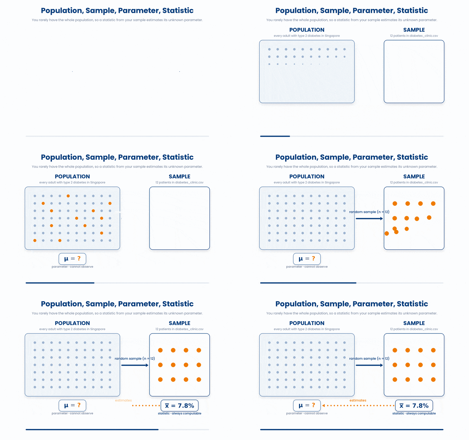
The whole game of inference is this: use the statistic you can compute to estimate the parameter you cannot. The sample mean is your best single guess at the population mean. Run the line below to compute that statistic from the clinic data.

library(readr)
clinic <- read_csv("diabetes_clinic.csv")
mean(clinic$hba1c, na.rm = TRUE)

Notice na.rm = TRUE. The hba1c column has two missing values. Leave it out and mean() returns NA, not a number — a silent trap whenever a clinical column has gaps.

Keep the two worlds straight.

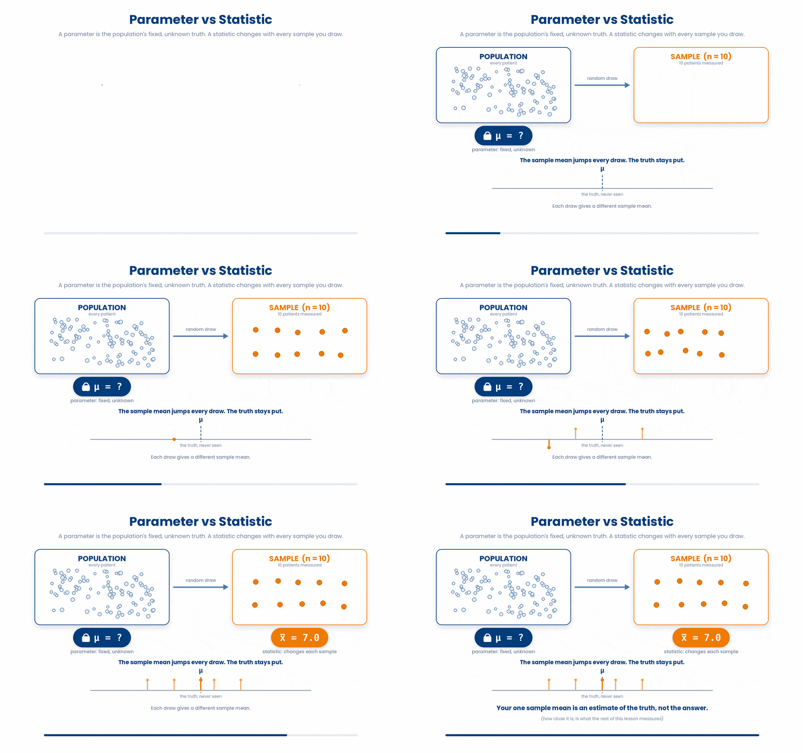
• A parameter is a fixed, unknown truth about the population.
• A statistic is a known number that changes with every sample you draw.

The novice trap is treating your one sample mean as the answer; it is only an estimate, and the rest of this lesson is about how good an estimate it is.

Your sample mean is one number, but it is not the only one you could have gotten. Draw a different twelve patients and you get a slightly different mean. The sampling distribution is the spread of a statistic across many imagined repeats of the very same study. It is the single idea underneath every confidence interval.

You never actually repeat a real study hundreds of times. But you can imagine it, and in R you can simulate it. Picture drawing a fresh sample, computing its mean, and writing that mean down — then doing it a thousand times. The thousand means have their own shape, centre, and spread.

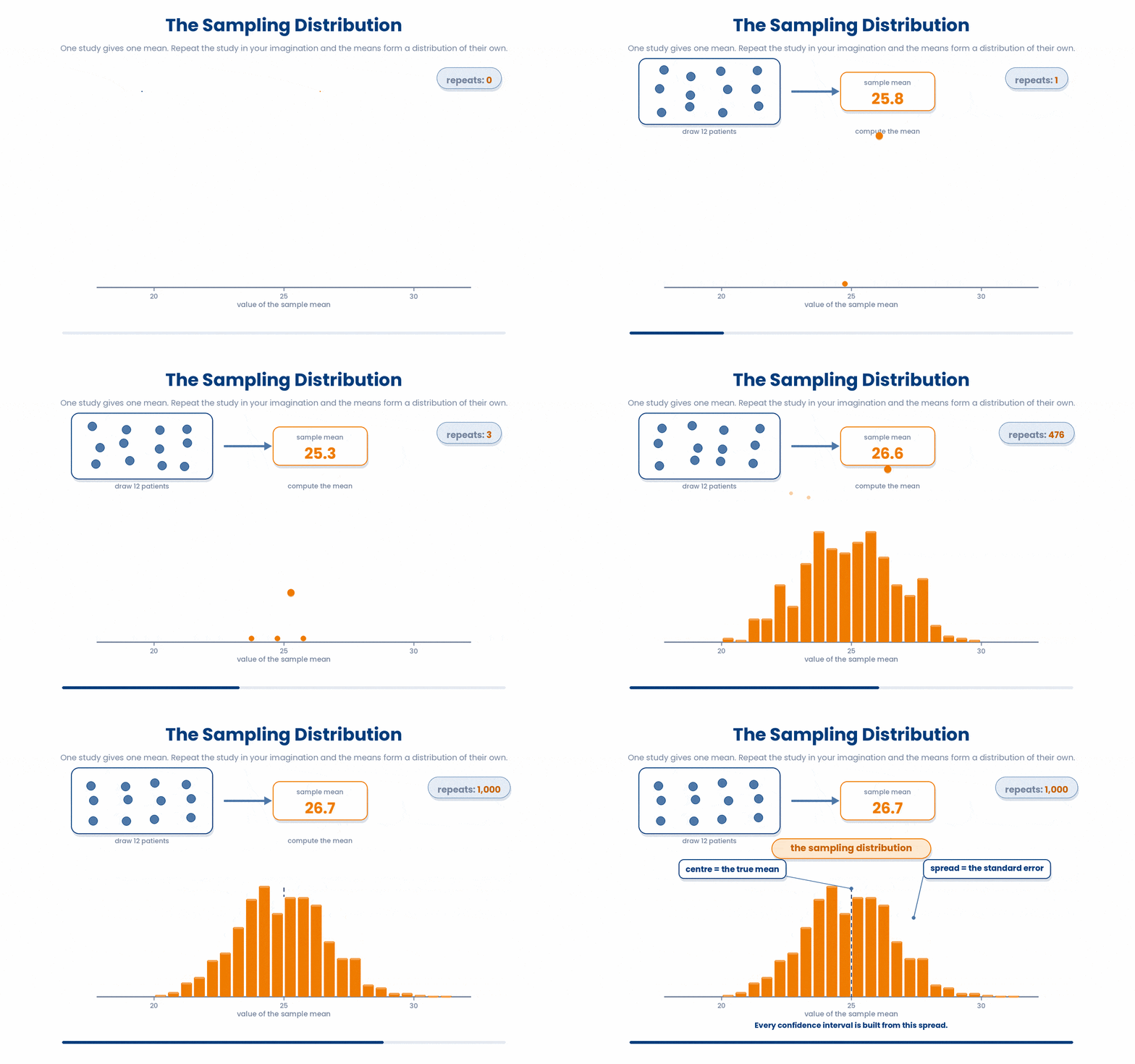
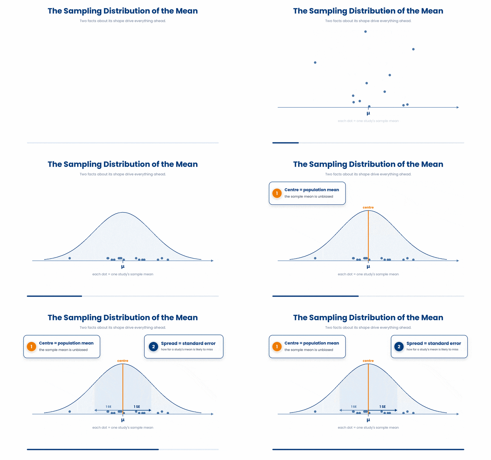
Two facts about that shape drive everything ahead. Its centre sits at the true population mean, so the sample mean is unbiased. Its spread tells you how much one study's mean is likely to miss by — and that spread has a name, the standard error, which is the next section.

The spread of that sampling distribution has a name. The standard error is the standard deviation of a statistic across repeated samples — in plain terms, how much your estimate would wobble if you ran the study again. It measures uncertainty in an estimate.

Do not confuse it with the standard deviation, which you met describing data: the SD measures how spread out the individual patients are. The SD is about people; the SE is about your estimate of their average.

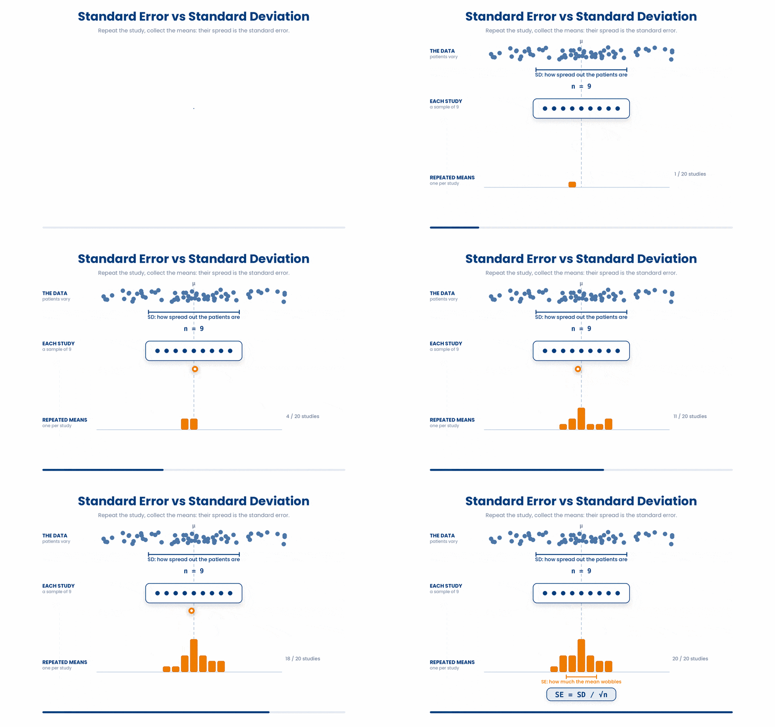
For a mean, the two are linked by a short formula: the standard error equals the sample SD divided by the square root of the sample size. In R that is sd(x) / sqrt(length(x)), where length(x) is the number of values.

hba1c <- c(7.2, 8.1, 6.5, 9.4, 7.8, 6.9, 8.4, 7.1)
se <- sd(hba1c) / sqrt(length(hba1c))
se

The square root in the denominator is the key. Quadruple your sample size and the SE halves, because the square root of four is two. So a bigger sample gives you a more precise estimate.

But notice what does not change. A bigger sample shrinks the SE, yet it leaves the SD essentially alone — patients are as different from each other in a big study as in a small one. The classic mistake is reporting the SD when you mean the SE, or expecting more data to shrink the SD; more data sharpens your estimate, not the spread of people.

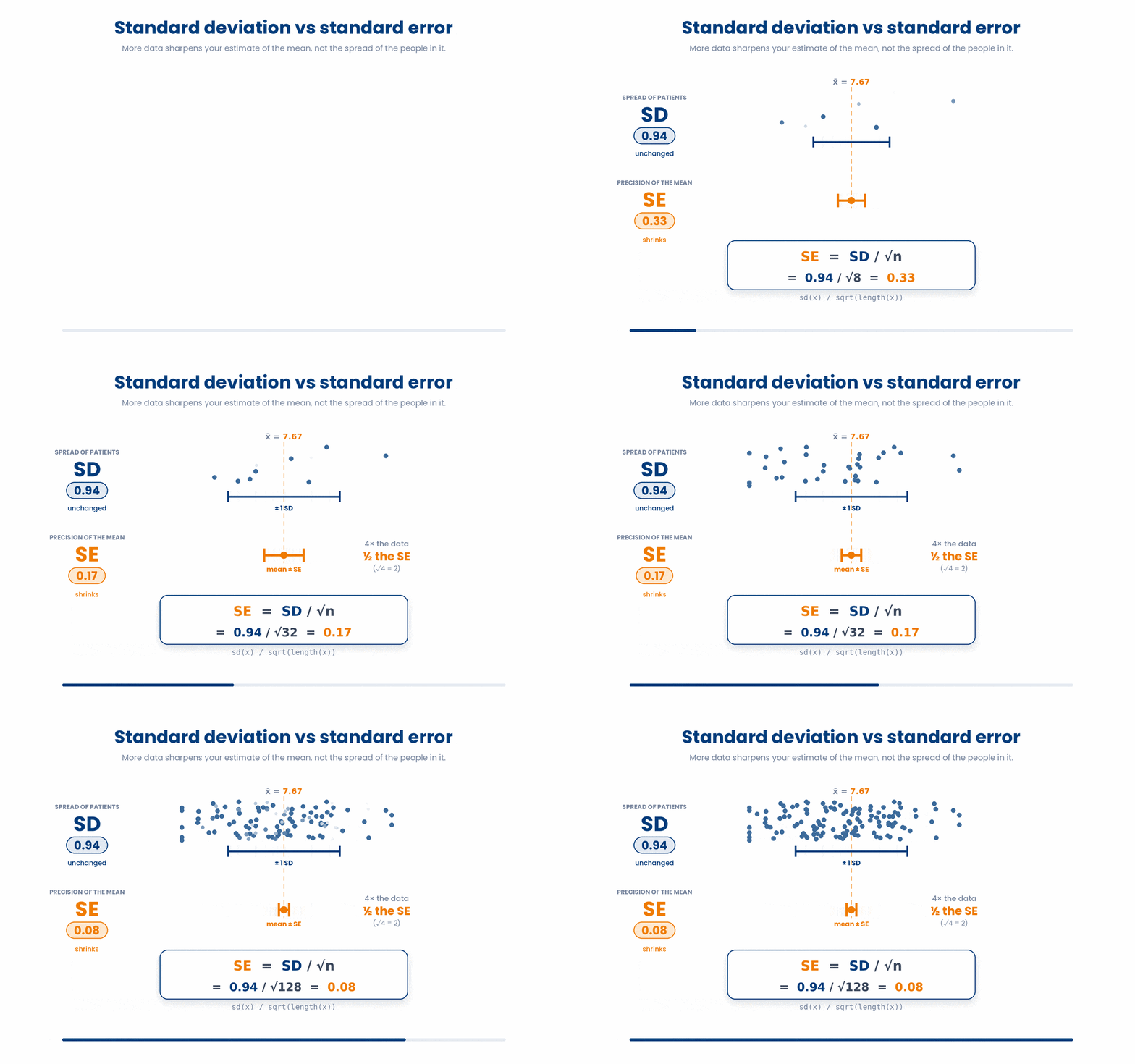
Plug numbers into the formula directly to feel it. If the SD is 10 and you have 100 patients, the SE is ten divided by the square root of a hundred — ten divided by ten.

Now, let’s try the worked example below and see precision grow with sample size.

sd_x <- 10
sd_x / sqrt(25)
sd_x / sqrt(100)

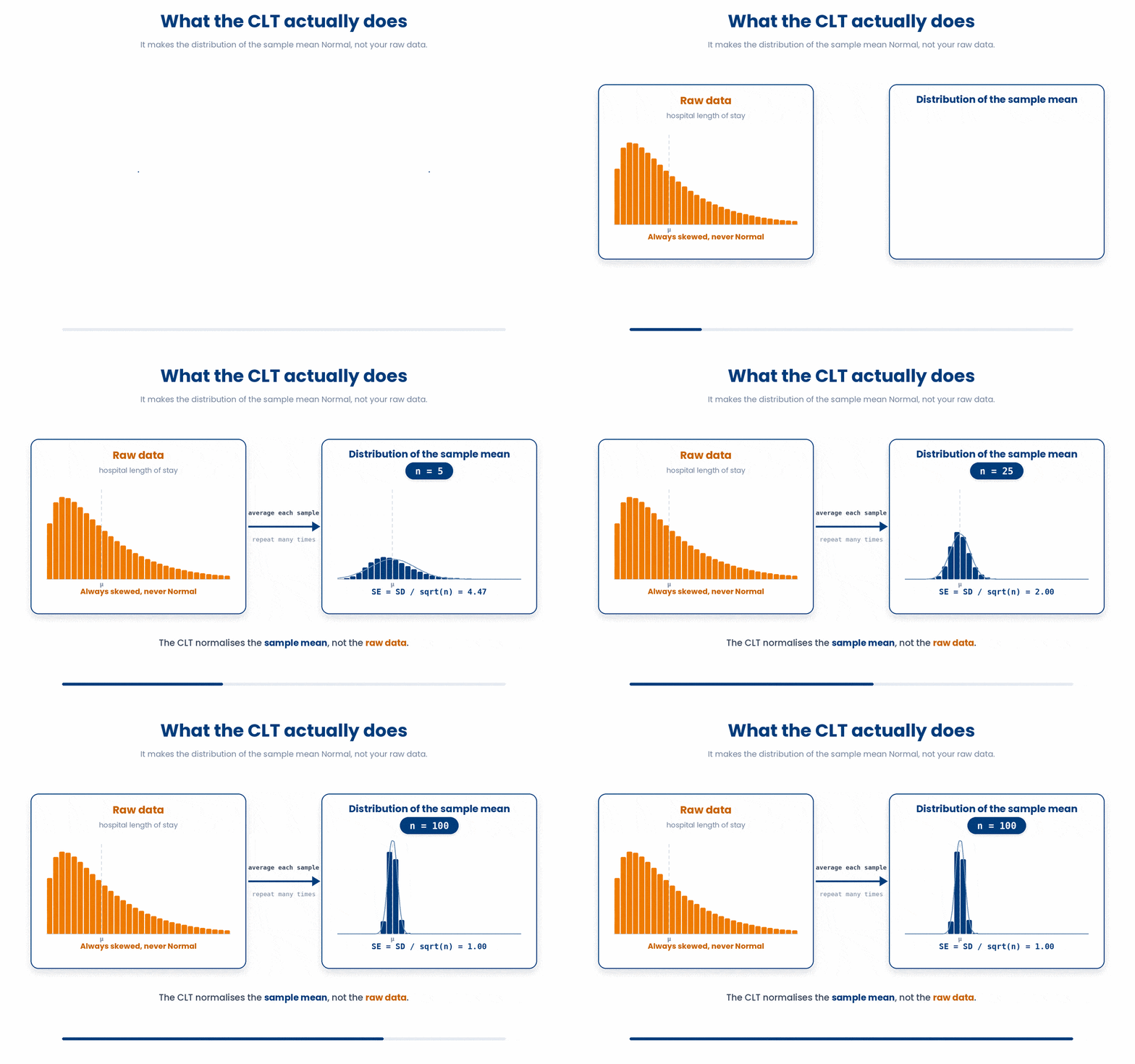
Now the payoff. The Central Limit Theorem says that as your sample size grows, the sampling distribution of the mean becomes Normal — bell-shaped — almost no matter how lopsided the raw data is. That is why the Normal curve from Module 4 powers confidence intervals for means even when individual patients are not Normal.

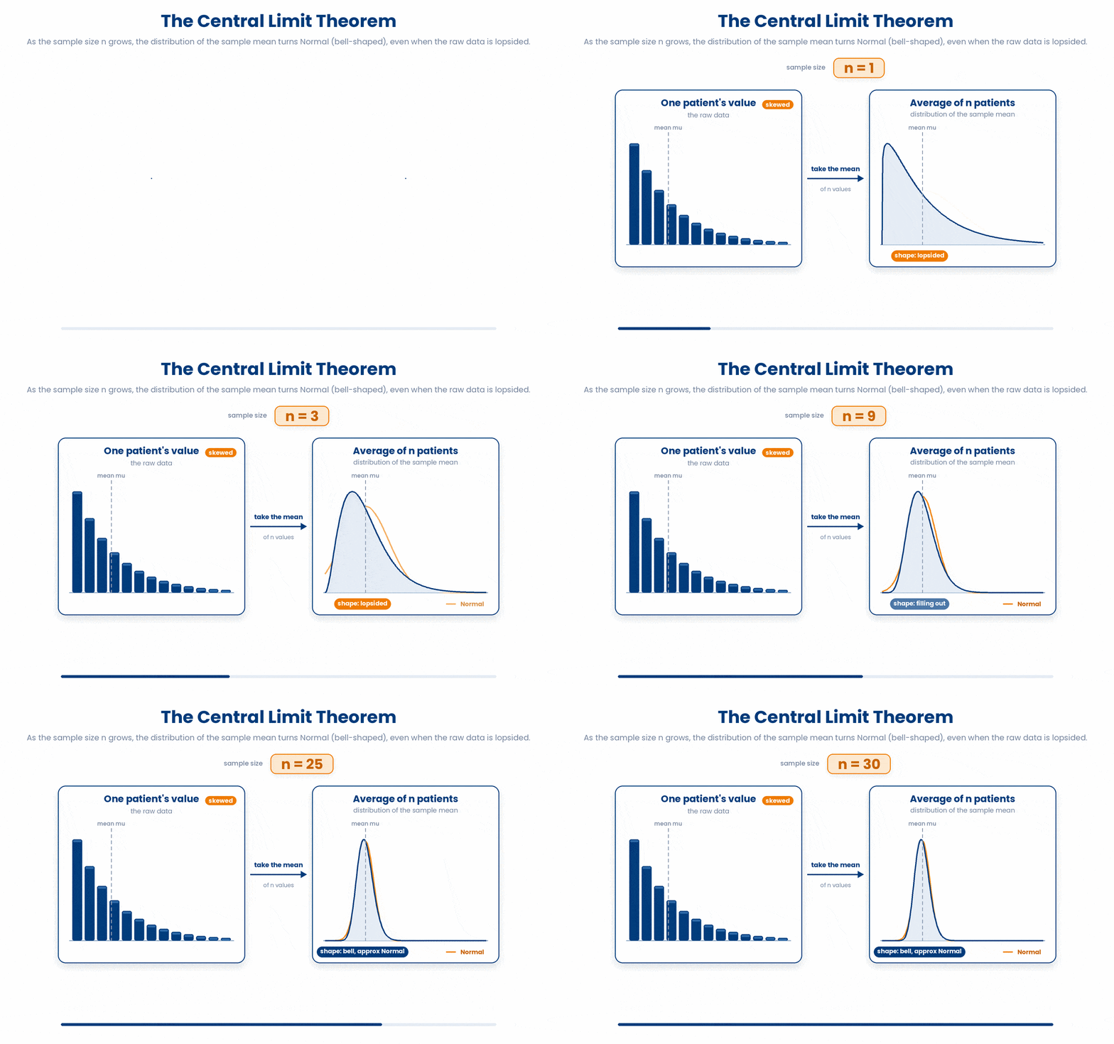
We will not prove it with algebra. We will watch it happen. Three tools build the simulation. sample() draws patients at random; replicate() repeats an action many times and collects the answers; set.seed() fixes the random number generator so your run matches the next person's exactly.

Hospital length of stay is famously right-skewed: most patients leave in a few days, a long tail stays for weeks. We simulate such a population with rexp, the exponential distribution, which is heavily skewed — the opposite of Normal.

library(ggplot2)
set.seed(2025)
los <- rexp(10000, rate = 1 / 5) # 10,000 individual stays: right-skewed
means <- replicate(10000, mean(rexp(30, rate = 1 / 5))) # mean of each 30-patient sample
d1 <- data.frame(v = los, panel = "1. Individual patients (skewed)")
d2 <- data.frame(v = means, panel = "2. Mean of 30 patients (Normal)")
d <- rbind(d1, d2)
ggplot(d, aes(v)) +
 geom_histogram(bins = 40, fill = "steelblue") +
 facet_wrap(~ panel, scales = "free") +
 labs(x = "Length of stay (days)", title = "The Central Limit Theorem in action")

That histogram is anything but a bell. Hold that picture: the raw data is skewed. Now watch what happens to the mean of a sample drawn from it.

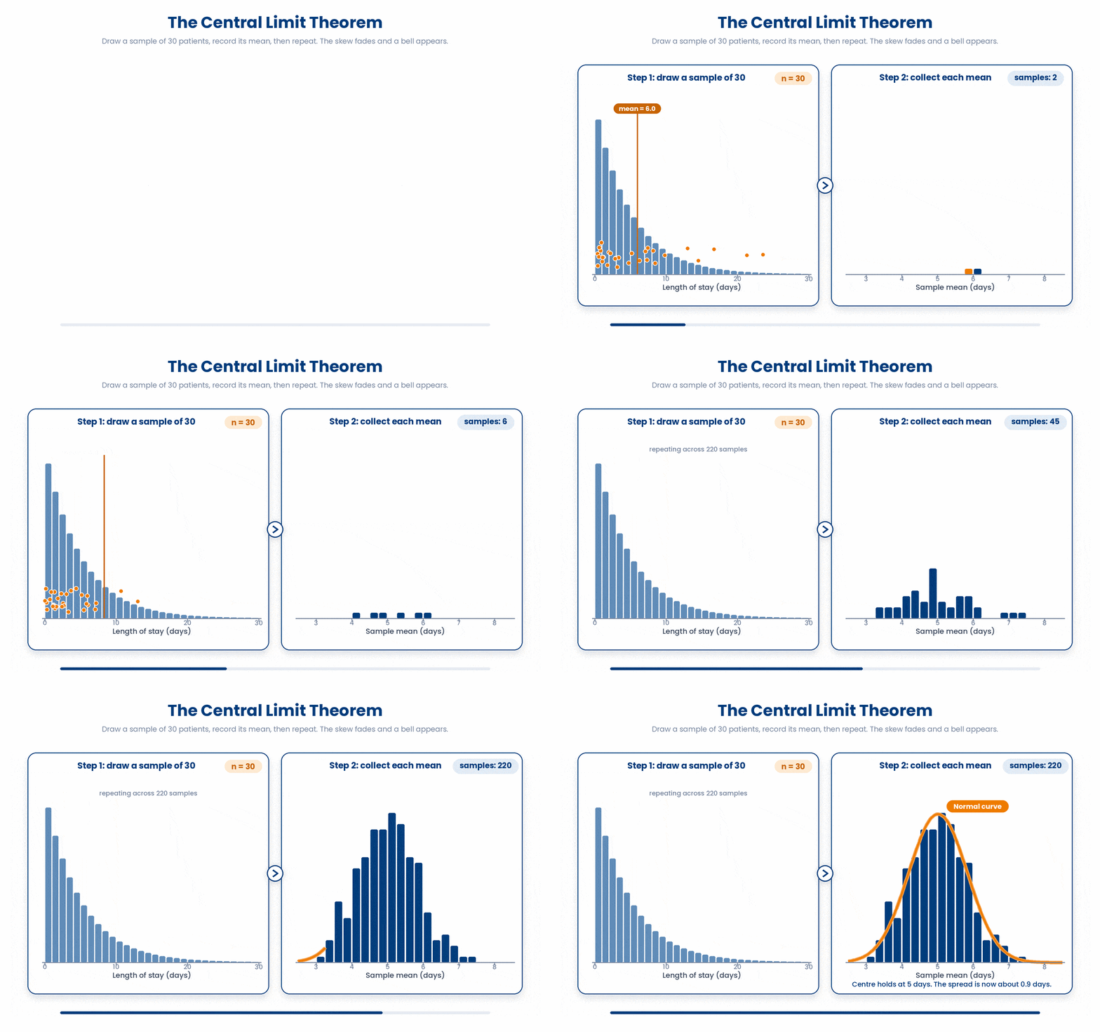
Here is the simulation in one block. Read it from the inside out: draw a sample of size n with sample(), take its mean, and let replicate() do that 2000 times. With n = 5 the means are still a little skewed; bump n to 50 and the histogram of means is a clean bell.

set.seed(2025)
los <- rexp(10000, rate = 1 / 5)
means_n50 <- replicate(2000, mean(sample(los, size = 5))) #try 5 and 50
ggplot(data.frame(means_n50), aes(means_n50)) +
  geom_histogram(bins = 40, fill = "darkorange") +
  labs(x = "Sample mean of length of stay", title = "Means go Normal (n = 50)")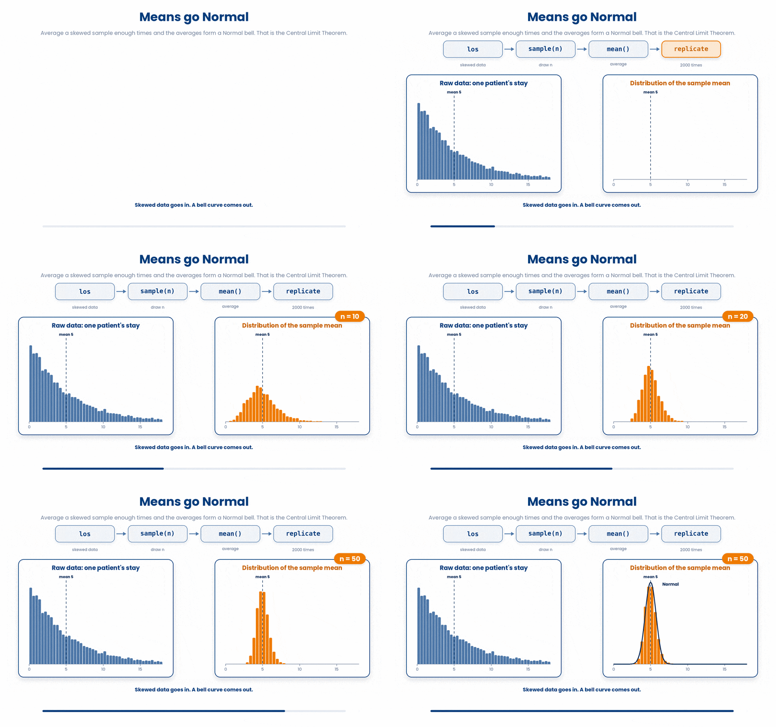

This is the trap the CLT is most often misread into. The CLT does NOT make your raw data Normal. The length-of-stay values are still skewed and always will be. What becomes Normal is the distribution of the sample mean. Confusing the two is the single most common error in this whole topic.

One more habit the simulation teaches. Re-running a simulation without set.seed() gives different numbers every time, so nobody can reproduce your figure. Set the seed once at the top, and your result is fixed. This is reproducibility, the same principle behind Quarto reports.

You have reached the end of the module. Try the same questions again — your answers here, paired with your pre-test answers, are how we measure what the module taught you. Answer every question and confidence rating, then click Submit and see results to view your score.

Here is how your post-test answers compare with your pre-test answers. The pre/post pairing is the most reliable way to see what this module actually taught you.