

1 Before you start
This is not graded, and it does not count towards anything. Answer every question even if you are only guessing — having a go at something before you have been taught it is one of the best ways to remember it afterwards. The lesson ends with another short check, and there you will be shown the correct answer for anything you missed. Choose an option for every question and confidence rating, then click Submit answers.
The positive predictive value (PPV) is computed from the 2x2 table by reading
A patient asks what a positive result means for them. Which probability answers that question?
A test has sensitivity 0.95. A patient tests positive and a colleague concludes there is a 95% chance of disease. What did the colleague confuse?
A test has a fixed sensitivity and specificity. You move it from a high-prevalence clinic to a low-prevalence screening population. What happens to its positive predictive value?
Using natural frequencies, a test with sensitivity 0.90 and specificity 0.92 screens 100,000 people at 1% prevalence: 900 true positives and 7,920 false positives. What is the PPV?
A screening test with sensitivity 0.90 and specificity 0.92 has a PPV of only about 0.10 at 1% prevalence. Why is the PPV so low?
You want sensitivity, specificity, PPV and NPV with 95% confidence intervals from a 2x2 table in R. Which function gives them?
You pass a 2x2 table to epi.tests() but put disease status in the rows and the test result in the columns. What is the likely consequence?
I can compute PPV and NPV across the test rows of a 2x2 table and explain why the chance of disease given a positive test is not the same as sensitivity.
I can use natural frequencies to walk from a prevalence to a PPV, and explain why a positive screen means little in a low-prevalence setting.
I can run epi.tests() from epiR on a correctly oriented 2x2 table to report sensitivity, specificity, PPV and NPV, each with a confidence interval.
2 Introduction
In Part I you built the 2x2 diagnostic table and read sensitivity and specificity down its disease columns — fixed properties of the test itself. But a patient does not know their true status; they hold a result and want the truth behind it. This part answers their question: my test came back positive, so how likely is it that I really have the disease?
This part of the module covers four steps, each one building on the last:
- PPV and NPV — what a result means for a patient, read across the test rows as P(disease | positive) and P(no disease | negative), never to be confused with sensitivity.
- Prevalence — why predictive values rise and fall with how common the disease is, even though the test never changes.
- Natural frequencies — imagining 100,000 whole people to walk from a prevalence to a post-test probability with counting, not algebra.
- Metrics in R — computing every measure at once, each with a confidence interval, using epi.tests() from the epiR package.
By the end of this part you will be able to compute PPV and NPV across the test rows, explain why the chance of disease given a positive test is not the same as sensitivity, reason in natural frequencies to find a PPV from a prevalence, and run epi.tests() to report every metric with a confidence interval — and say plainly why a positive screen in a low-prevalence setting means far less than students expect.
Try every snippet in the R Scratchpad on the right. This part needs no data file — you will build the small screening tables yourself with matrix() and c(), and load the epiR package with library(epiR).
3 PPV and NPV: what a result means for a patient
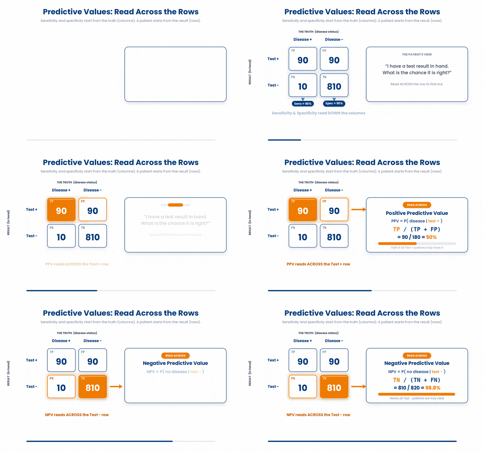
Sensitivity and specificity start from the truth and look at the test. A patient sits at the opposite end: they have a result in hand and want to know the truth. For that you read ACROSS the test rows instead of down the disease columns.
The positive predictive value (PPV) is the chance a patient truly has the disease given a positive test: P(disease | positive). You condition on the test, so you read across the Test = Positive row: TP / (TP + FP). The negative predictive value (NPV) is the chance a patient is truly disease-free given a negative test: P(no disease | negative), read across the Test = Negative row as TN / (TN + FN).
Now the trap that catches every beginner, and the whole reason this part exists. P(positive | disease) and P(disease | positive) are different questions with different answers. Sensitivity reads down the disease column; PPV reads across the test row. Swapping them — assuming a positive result means the patient almost certainly has the disease — is the classic diagnostic error.
Compute both predictive values by hand from the same four counts — reading ACROSS the test rows this time, not down the disease columns.
Try this snippet in the R Scratchpad on the right.
tp <- 90
fp <- 7
fn <- 10
tn <- 93
ppv <- tp / (tp + fp)
npv <- tn / (tn + fn)
c(PPV = ppv, NPV = npv)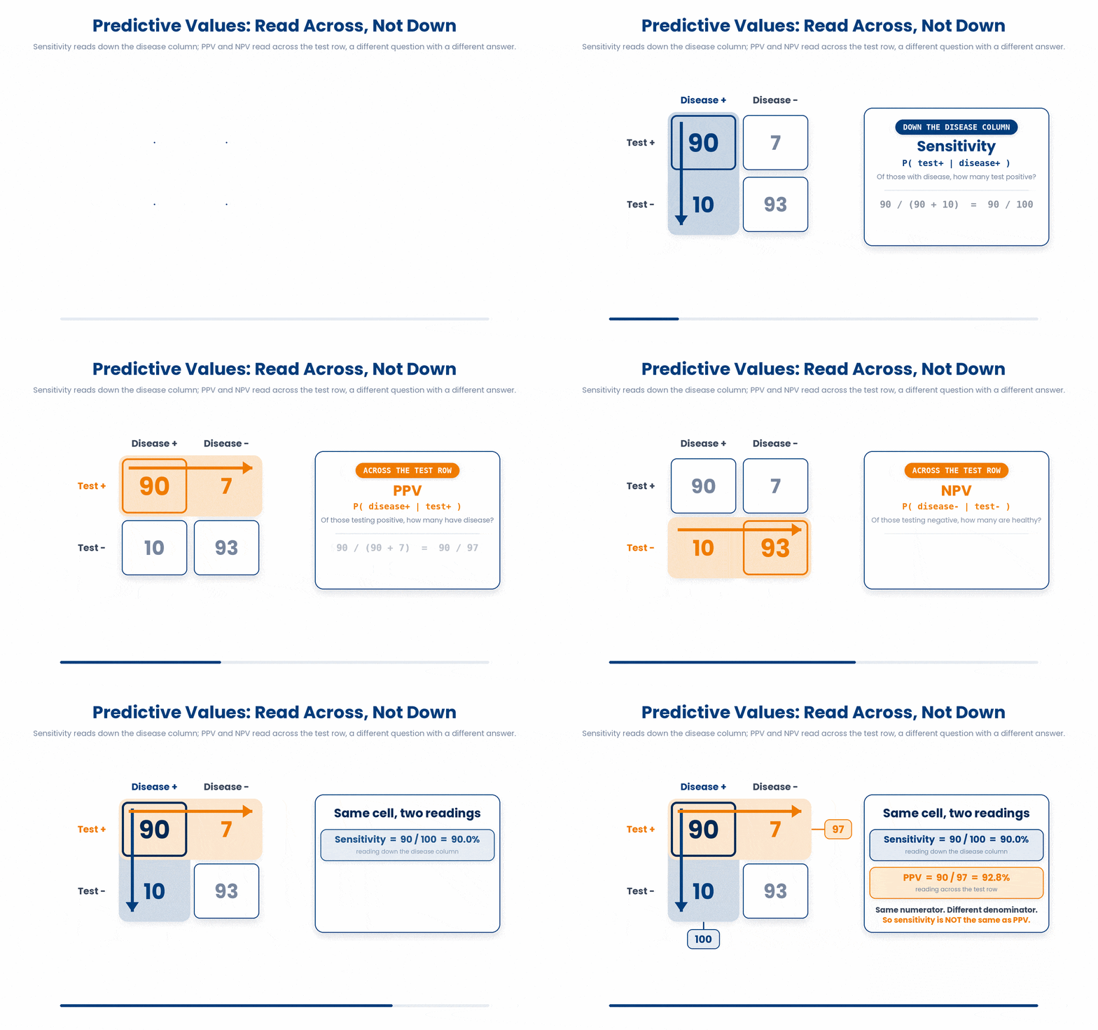
3.1 Why PPV moves with prevalence
Unlike sensitivity, PPV and NPV depend on prevalence — how common the disease is in the population you are testing. The reason is the false positives. In a low-prevalence setting there are very few diseased people but a vast pool of healthy people, so even a small false-positive rate produces a flood of false alarms that swamp the true ones.
This is why the same excellent test gives a high PPV in a specialist clinic full of sick patients but a low PPV when used to screen the general population. A good sensitivity and specificity do NOT guarantee a high PPV — prevalence has the final say. We make this concrete with natural frequencies next.

4 Natural frequencies: reasoning with whole people
The cleanest way to find a PPV is not algebra — it is to imagine a large, round group of people and count. This is the natural-frequency method, and it turns a confusing probability problem into simple arithmetic on whole patients.
The recipe has three steps. First, the pre-test probability is just the prevalence — the chance a patient has the disease before any test. Imagine a population of that size, say 100,000. Split it into diseased and healthy using the prevalence. Then apply sensitivity to the diseased group and specificity to the healthy group to fill the four cells. The post-test probability after a positive result is then just the PPV you read off the counts.
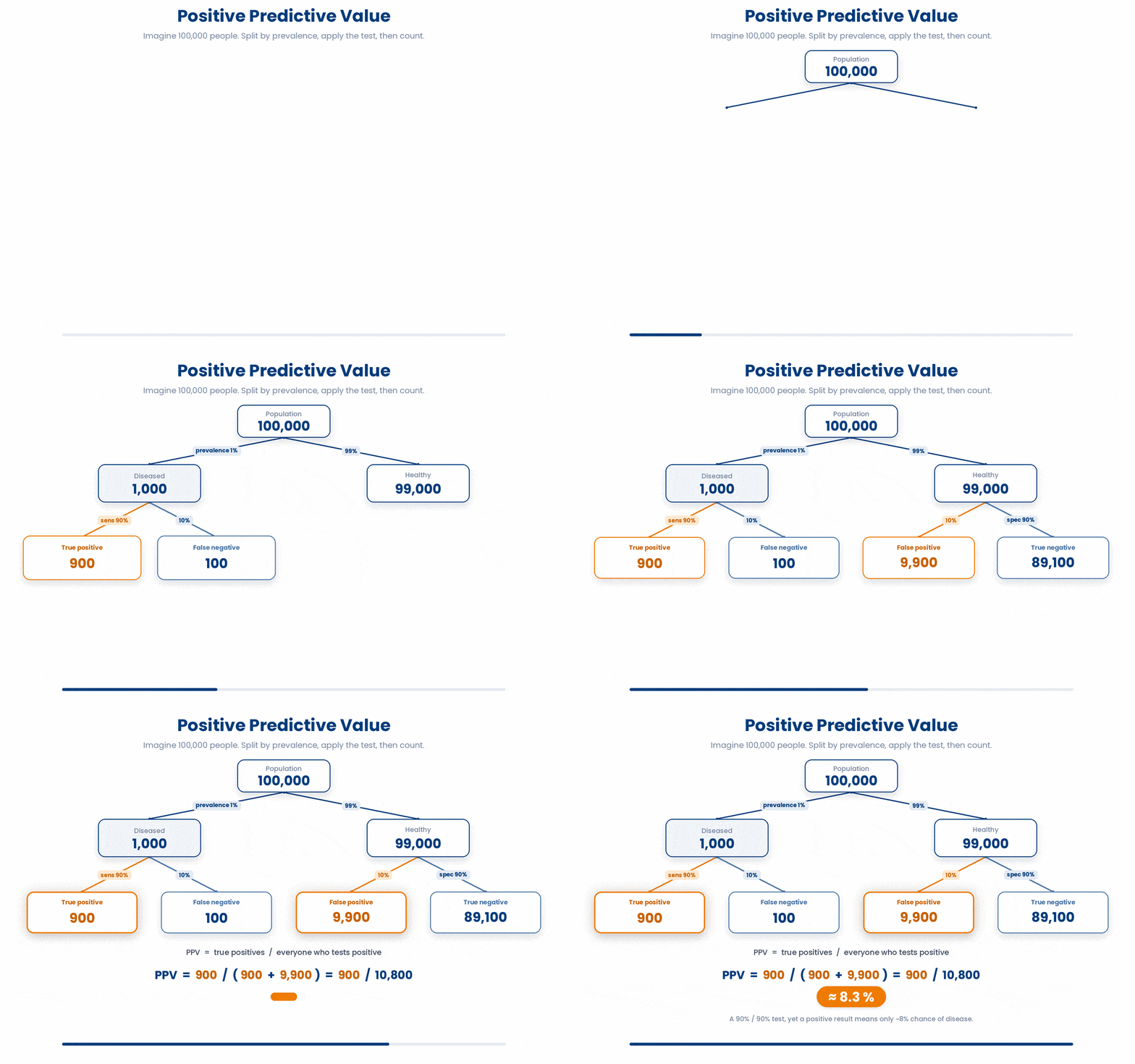
Work an example. A test has sensitivity 0.90 and specificity 0.92, used to screen a population where prevalence is 1% (so 1 in 100). Out of 100,000 people, 1,000 have the disease and 99,000 do not.
- Of the 1,000 diseased, sensitivity 0.90 makes 900 test positive (true positives) and 100 test negative (false negatives).
- Of the 99,000 healthy, specificity 0.92 clears 91,080 as negative (true negatives), leaving 8% — that is 7,920 — testing positive (false positives).
Now find the PPV by reading across the positive row. The positives are 900 true plus 7,920 false, a total of 8,820. The PPV is 900 / 8,820, which is about 0.10. Even with a 90% sensitivity, a positive screen here carries only a 1-in-10 chance of real disease — because the 7,920 false alarms vastly outnumber the 900 real cases.
Try this snippet in the R Scratchpad on the right.
n <- 100000
prevalence <- 0.01
sensitivity <- 0.90
specificity <- 0.92
diseased <- n * prevalence
healthy <- n - diseased
tp <- diseased * sensitivity
fp <- healthy * (1 - specificity)
ppv <- tp / (tp + fp)
ppv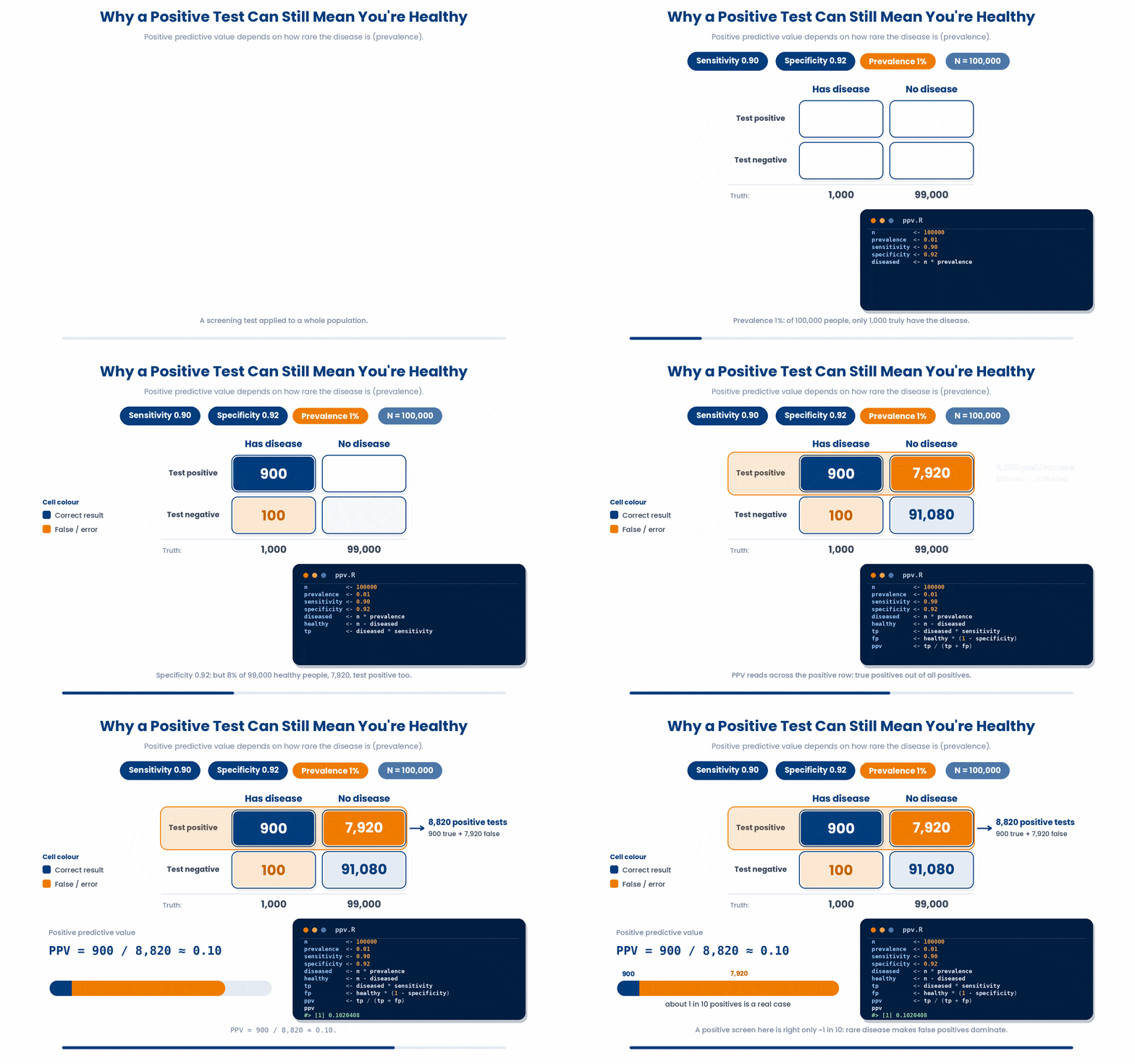
Sit with that number. Even an excellent test gives a low PPV when prevalence is low, because false positives drawn from the huge healthy majority drown out the few true positives. This is the single most important idea in screening, and the reason a positive screen is usually followed by a confirmatory test, not a diagnosis.
Raise the prevalence and the PPV climbs. Take the very same test to a clinic where 10% of patients have the disease. Out of 100,000 there are now 10,000 diseased (9,000 true positives) and 90,000 healthy (7,200 false positives), so the PPV jumps to 9000 / (9000 + 7200), about 0.56. Same test, prevalence up tenfold, PPV from one-in-ten to better than even.
Try this snippet in the R Scratchpad on the right.
n <- 100000
prevalence <- 0.10
sensitivity <- 0.90
specificity <- 0.92
diseased <- n * prevalence
healthy <- n - diseased
tp <- diseased * sensitivity
fp <- healthy * (1 - specificity)
ppv <- tp / (tp + fp)
ppv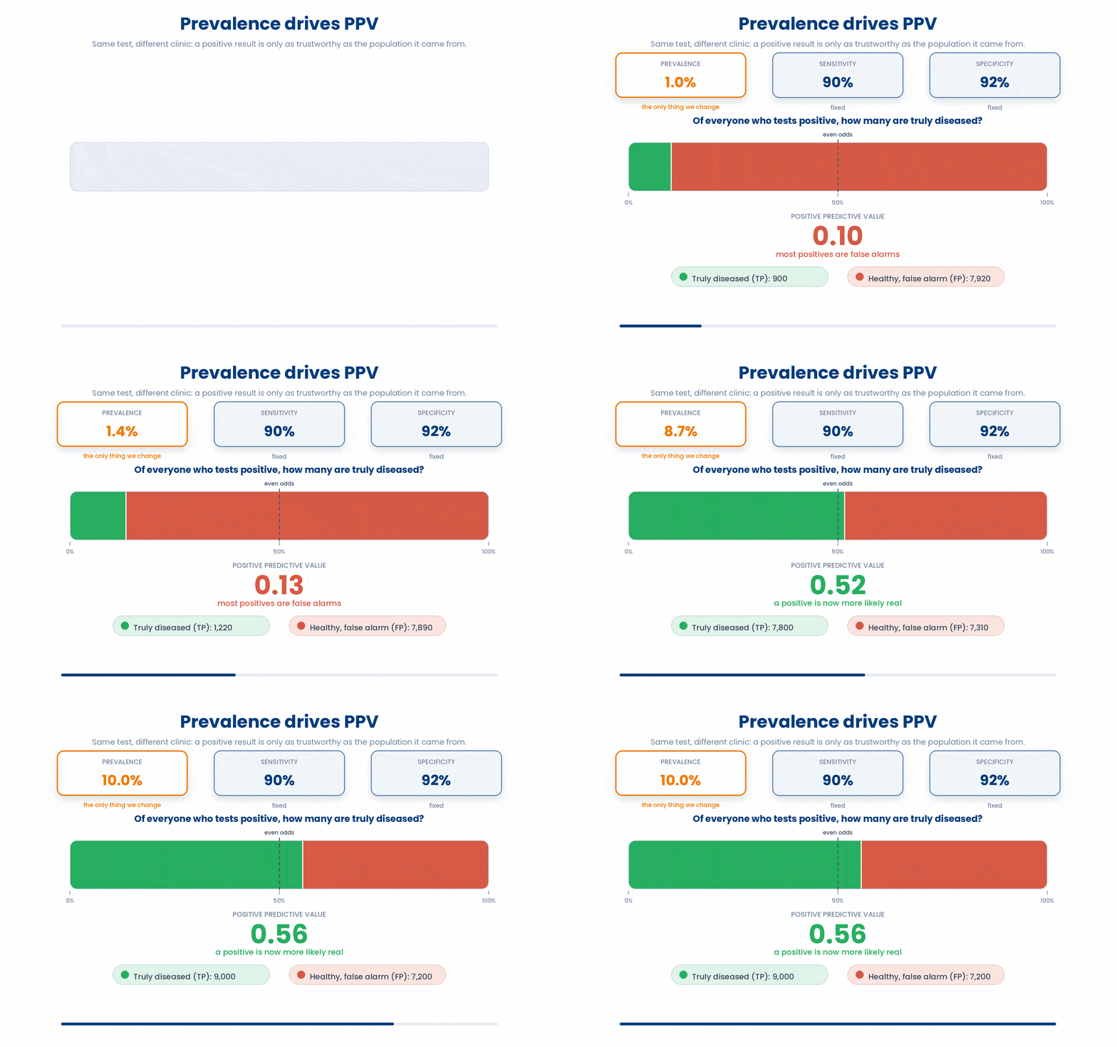
5 Computing every metric with epi.tests()
Hand arithmetic is good for understanding, but in practice you let R compute every metric at once, complete with confidence intervals. The tool is epi.tests() from the epiR package.
The epiR package is a collection of veterinary and human epidemiology functions; switch it on with library(epiR). Its epi.tests function takes a 2x2 table and returns sensitivity, specificity, PPV, NPV and more, each with a 95% confidence interval.
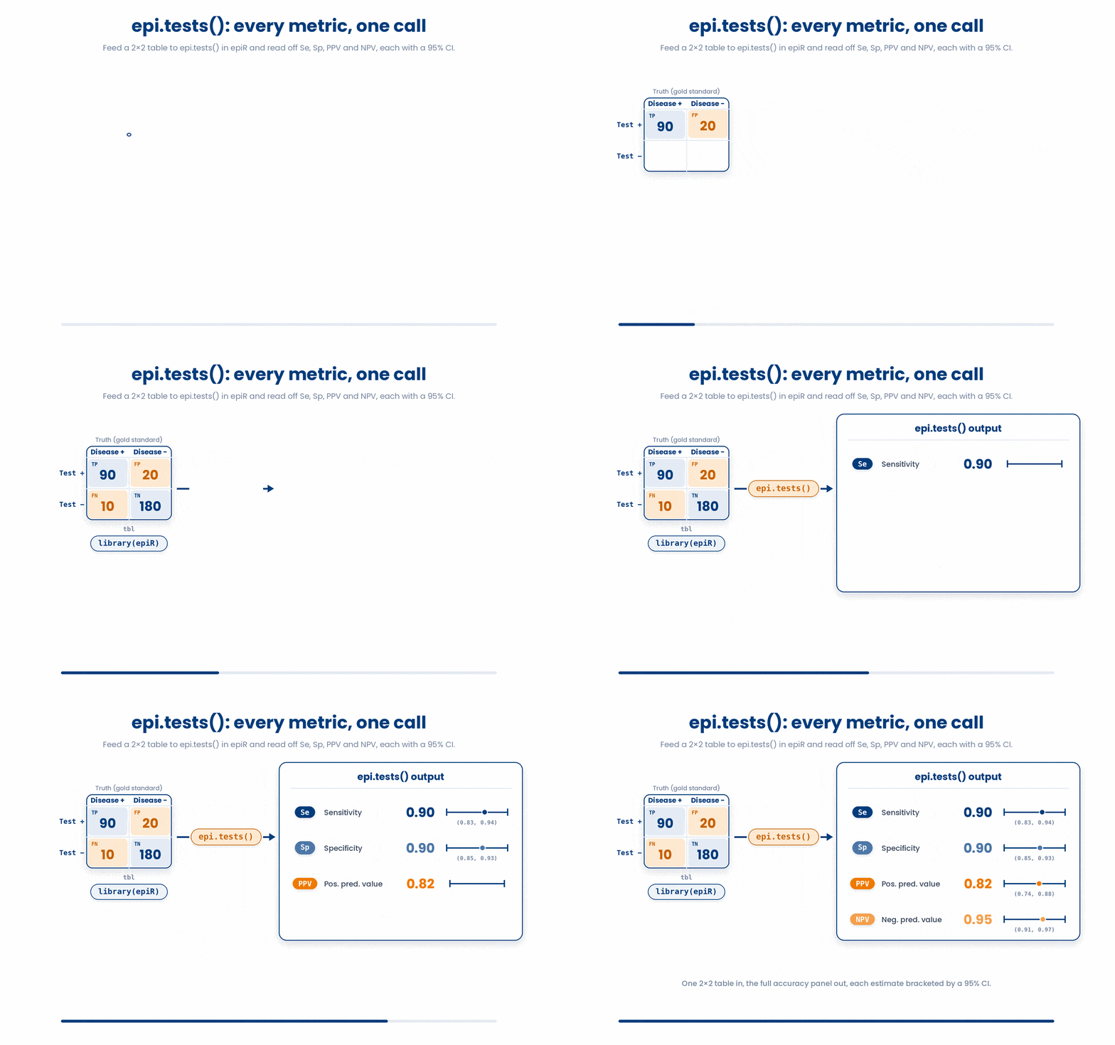
There is one rule you must obey, and getting it wrong is the most common mistake with this function. epi.tests() expects the test outcome in the ROWS and the true disease status in the COLUMNS, with the positive/diseased cell at the top left. Feed it a table in the wrong orientation and it will silently compute the metrics for the wrong cells. Always print the table and check its dimnames before you trust the output.
Build the screening table from the natural-frequency counts — 900 true positives, 7,920 false positives, 100 false negatives, 91,080 true negatives — with the test in rows and disease in columns, then pass it in.
Try this snippet in the R Scratchpad on the right.
library(epiR)
dat <- c(900, 7920, 100, 91080)
screen_tab <- matrix(dat, nrow = 2, byrow = TRUE,
              dimnames = list(Test = c("Positive", "Negative"),
                              Disease = c("Yes", "No")))
screen_tab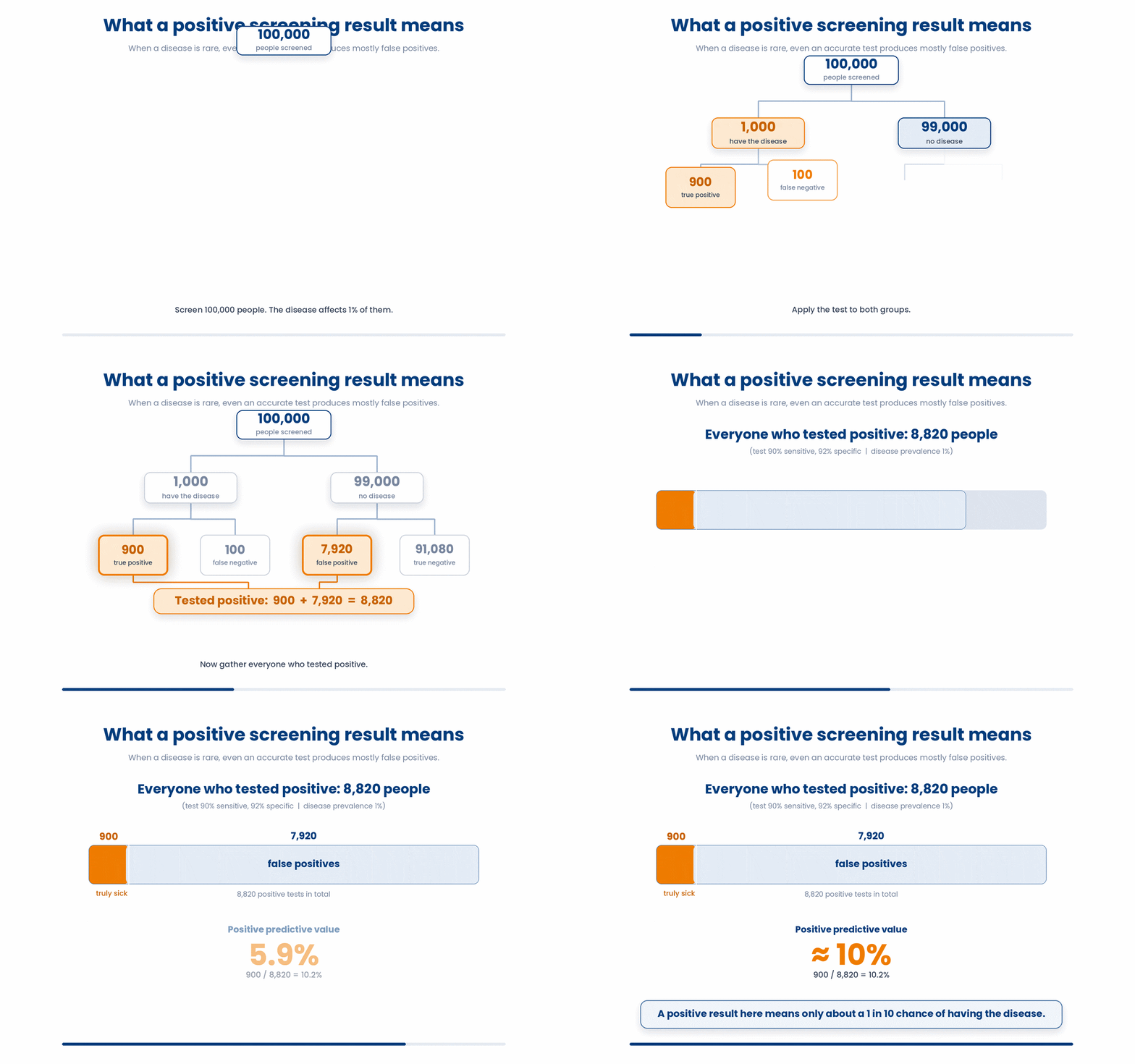
Now run the analysis. Read the output table for the rows labelled Sensitivity, Specificity, Pos. predict. value and Neg. predict. value — each shows the estimate with its confidence interval. The PPV will read about 0.10, exactly the number you counted by hand.
Try this snippet in the R Scratchpad on the right.
library(epiR)
dat <- c(900, 7920, 100, 91080)
screen_tab <- matrix(dat, nrow = 2, byrow = TRUE,
              dimnames = list(Test = c("Positive", "Negative"),
                              Disease = c("Yes", "No")))
epi.tests(screen_tab)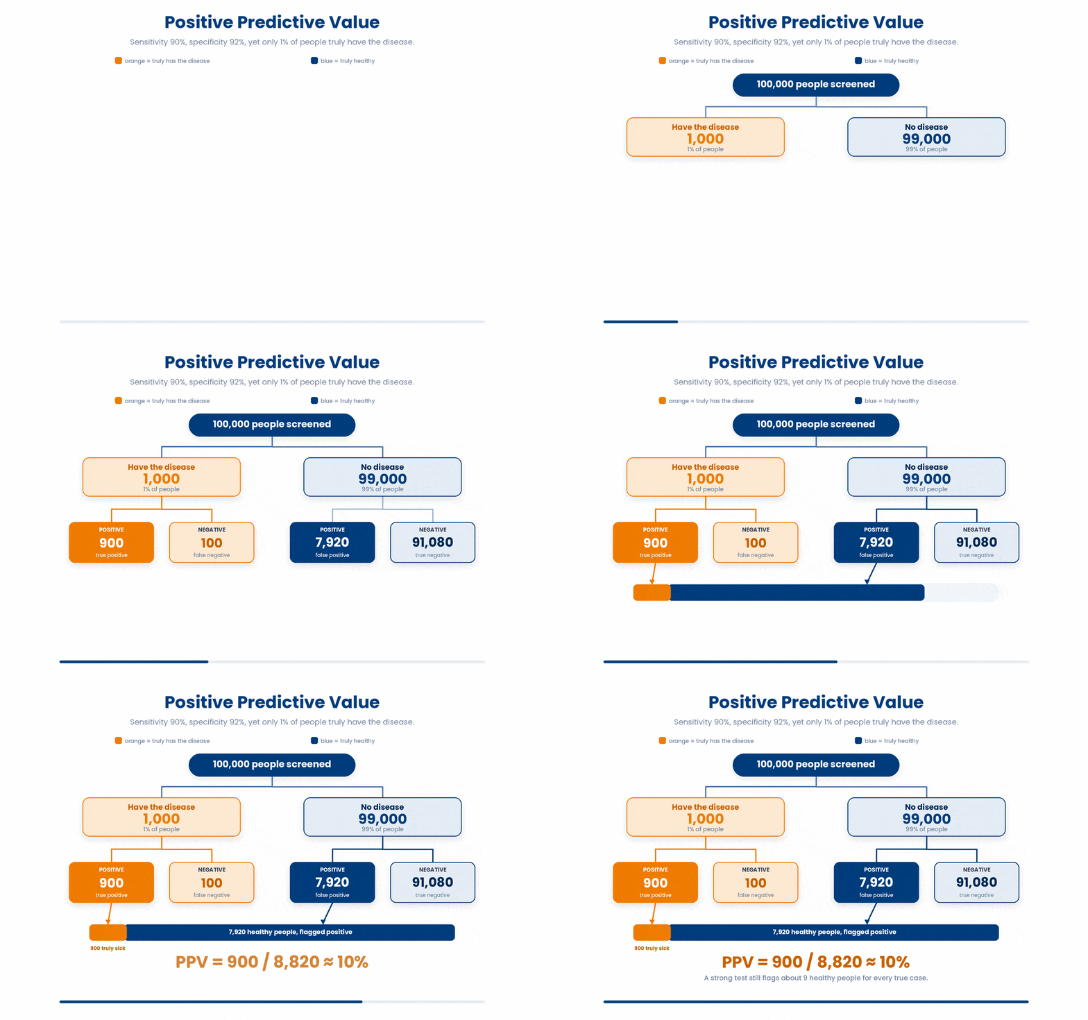
Notice what just happened. epi.tests() agreed with your natural-frequency count: a PPV near 0.10 for a test with 0.90 sensitivity. That is the punchline of the whole part — even an excellent test gives a positive result that means little in a low-prevalence screening setting, and R confirms it with a confidence interval to report.
6 Put it together
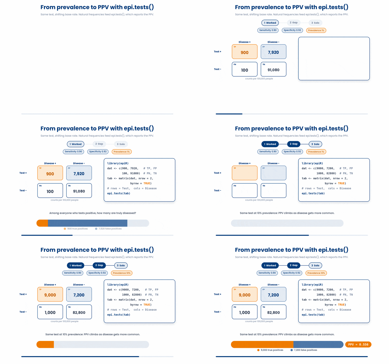
Now run the full chain on a fresh screening scenario: turn a prevalence and a test's sensitivity and specificity into natural-frequency counts, feed them to epi.tests(), and read the PPV. The worked example fades its support — study the full solution, fill the gap, then solve one alone.
Work through this example in three stages. You unlock each stage only after the tutor confirms the previous one. Each stage removes more of the scaffolding — by the end you are writing it yourself.
Problem: A screening test has sensitivity 0.90 and specificity 0.92 and is used where prevalence is 1%. Out of 100,000 people that is 1,000 diseased (900 true positives, 100 false negatives) and 99,000 healthy (91,080 true negatives, 7,920 false positives). Build the 2x2 table with test in rows and disease in columns, then read the PPV.
library(epiR)
dat <- c(900, 7920, 100, 91080)
tab <- matrix(dat, nrow = 2, byrow = TRUE,
              dimnames = list(Test = c("Positive", "Negative"),
                              Disease = c("Yes", "No")))
epi.tests(tab)- Order the four counts as TP, FP, FN, TN to match a row-wise 2x2
- byrow = TRUE fills the grid in that order, test in rows, disease in columns
- epi.tests() reports the PPV row near 0.10, swamped by false positives
The same solution with key parts replaced by ???.
Fill in every ??? so the code matches the reference,
then ask the tutor to check it.
Your turn: Now do the SAME test (sensitivity 0.90, specificity 0.92) at a higher prevalence of 10%. Out of 100,000 that is 10,000 diseased (9,000 true positives, 1,000 false negatives) and 90,000 healthy (82,800 true negatives, 7,200 false positives). Build the table and read the PPV by hand from 9000 / (9000 + 7200).
7 Check your understanding
You have reached the end of the module. Try the same questions again — your answers here, paired with your pre-test answers, are how we measure what the module taught you. Answer every question and confidence rating, then click Submit and see results to view your score.
The positive predictive value (PPV) is computed from the 2x2 table by reading
A patient asks what a positive result means for them. Which probability answers that question?
A test has sensitivity 0.95. A patient tests positive and a colleague concludes there is a 95% chance of disease. What did the colleague confuse?
A test has a fixed sensitivity and specificity. You move it from a high-prevalence clinic to a low-prevalence screening population. What happens to its positive predictive value?
Using natural frequencies, a test with sensitivity 0.90 and specificity 0.92 screens 100,000 people at 1% prevalence: 900 true positives and 7,920 false positives. What is the PPV?
A screening test with sensitivity 0.90 and specificity 0.92 has a PPV of only about 0.10 at 1% prevalence. Why is the PPV so low?
You want sensitivity, specificity, PPV and NPV with 95% confidence intervals from a 2x2 table in R. Which function gives them?
You pass a 2x2 table to epi.tests() but put disease status in the rows and the test result in the columns. What is the likely consequence?
I can compute PPV and NPV across the test rows of a 2x2 table and explain why the chance of disease given a positive test is not the same as sensitivity.
I can use natural frequencies to walk from a prevalence to a PPV, and explain why a positive screen means little in a low-prevalence setting.
I can run epi.tests() from epiR on a correctly oriented 2x2 table to report sensitivity, specificity, PPV and NPV, each with a confidence interval.
8 Your results
Here is how your post-test answers compare with your pre-test answers. The pre/post pairing is the most reliable way to see what this module actually taught you.
Submit the post-test to see your results.
What is the one thing from this module that is still unclear to you?