Diagnostic Tests and Bayes — Part I: The 2x2 Table, Sensitivity, and Specificity

Before you begin, take a few minutes to check what you already know and how confident you feel. You will see the same questions again at the end of the module — this helps both you and us measure what you have learned. Click an option for every question and confidence rating, then click Next to continue.

Earlier you met conditional probability — the chance of one event once you already know another, written P(A | B). Every diagnostic-test calculation is that idea made concrete: you take what you know about a patient and ask how the test behaves. This part builds the small table that all of those calculations start from, and reads the first two metrics off it.

This part of the module covers two foundations, the second building on the first:

• The 2x2 diagnostic table — the four counts (true positive, false positive, false negative, true negative) that every test metric is built from, laid out in R.
• Sensitivity and specificity — fixed properties of the test itself, read down the disease columns and unchanged by how common the disease is.

By the end of this part you will be able to name the four cells of a 2x2 table, build the table with matrix() (remembering byrow = TRUE), label it with dimnames and add totals with addmargins(), and read sensitivity and specificity down the disease columns — and explain why those two numbers do not change when prevalence does.

Try every snippet in the R Scratchpad on the right. This part needs no data file — you will build the small tables yourself with matrix() and c().

Every diagnostic-test calculation starts from one small table. You cross the test result (positive or negative) against the truth (disease present or absent), and count how many patients fall in each of the four cells. That is the whole foundation — get the four counts right and every metric follows.

Each cell has a name that says whether the test got it right:

• true positive (TP) — the test says positive and the disease really is present. A correct alarm.
• false positive (FP) — the test says positive but the disease is absent. A false alarm.
• false negative (FN) — the test says negative but the disease is present. A missed case.
• true negative (TN) — the test says negative and the disease really is absent. A correct all-clear.

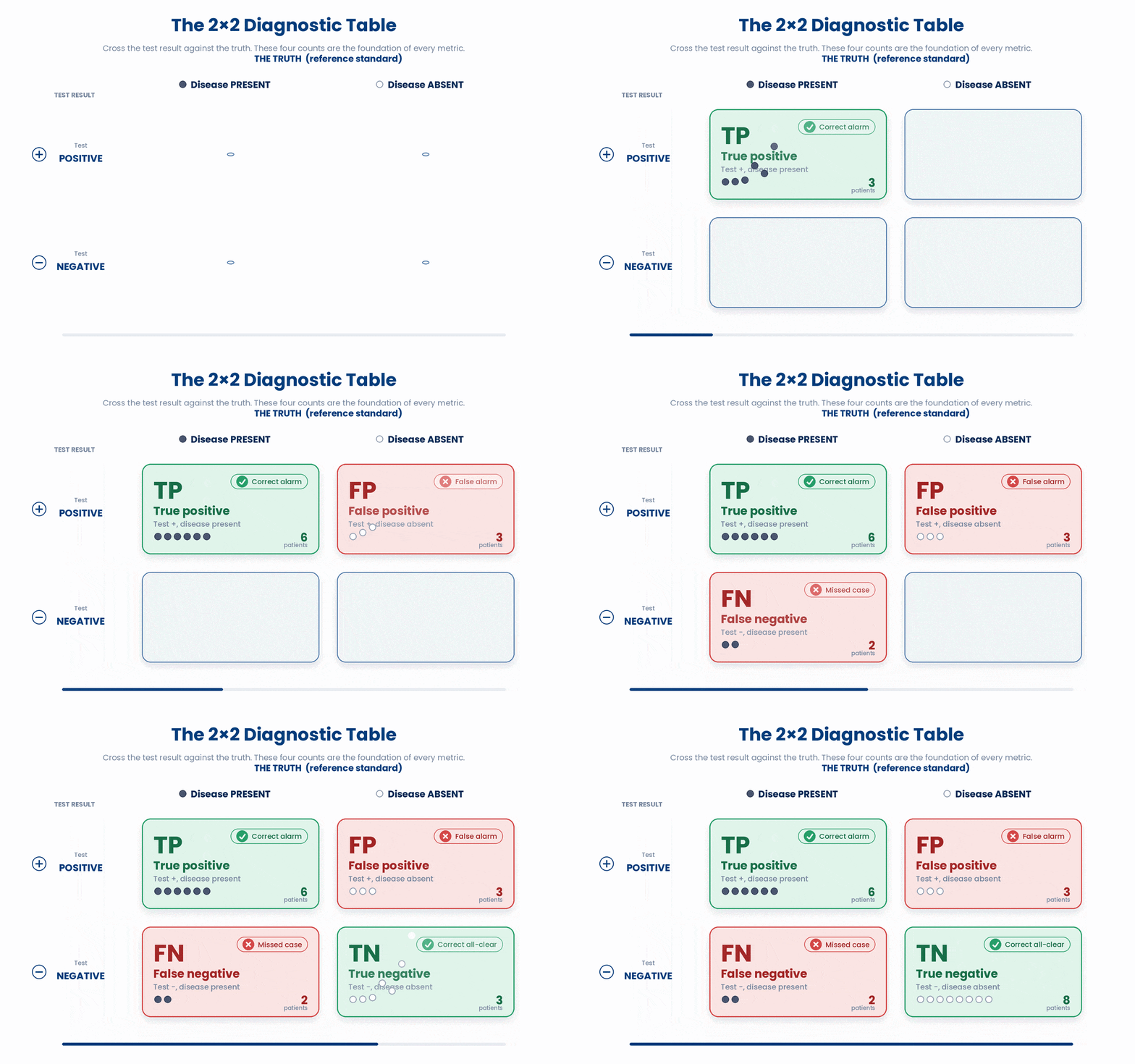
The word true or false tells you whether the test was correct; the word positive or negative tells you what the test said. So a false negative is a negative result that was wrong — the dangerous miss that sends a sick patient home.

You lay the four counts into a 2x2 grid with matrix(). Give it the four numbers, tell it how many rows with nrow = 2, and — this is the part beginners skip — set byrow = TRUE so R fills the grid row by row in the order you wrote them, not down the columns.

Suppose 90 patients have a positive test and disease (TP), 7 have a positive test but no disease (FP), 10 test negative yet have disease (FN), and 93 test negative with no disease (TN). Lay them out with the test in the rows and the disease in the columns.

counts <- c(90, 7, 10, 93)
tab <- matrix(counts, nrow = 2, byrow = TRUE)
tab

A bare table of numbers is hard to read, so label it. Set dimnames to name the rows and columns, and add row and column totals with addmargins — it appends a Sum row and a Sum column so you can see the margins at a glance.

counts <- c(90, 7, 10, 93)
tab <- matrix(counts, nrow = 2, byrow = TRUE)
dimnames(tab) <- list(Test = c("Positive", "Negative"),
                       Disease = c("Yes", "No"))
addmargins(tab)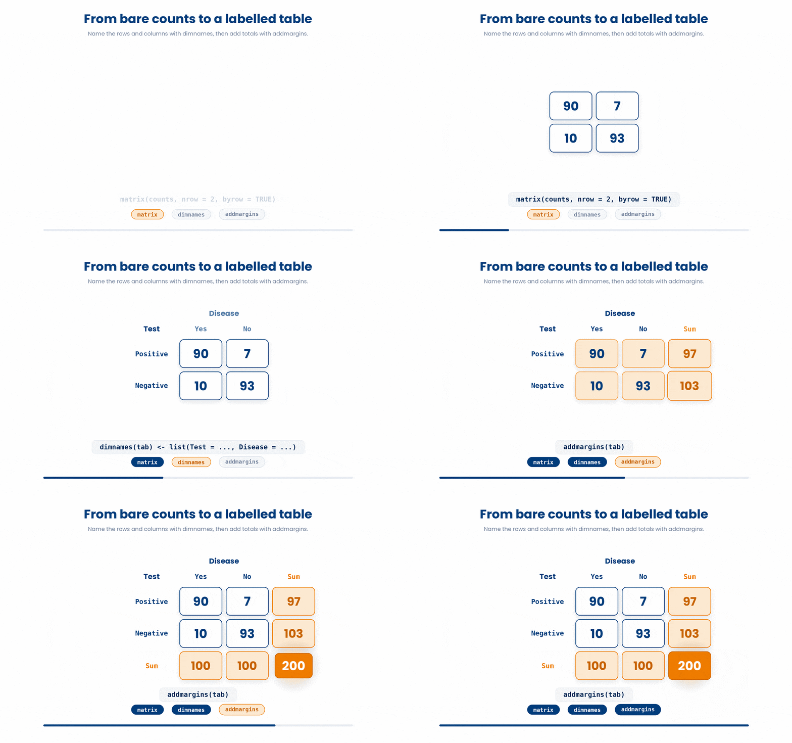

Read the margins to sanity-check. The Disease = Yes column sums to 100 diseased patients (90 + 10), and the Test = Positive row sums to 97 positives (90 + 7). Knowing which margin is which is the key to everything that follows.

With the table built, the first two metrics describe the test itself. You read them DOWN the disease columns — start from patients whose true status you already know, and ask how often the test agrees.

The sensitivity is the proportion of truly diseased patients the test correctly flags as positive. In symbols it is P(positive | disease) — you condition on disease, so you read down the Disease = Yes column: TP / (TP + FN). A sensitive test misses few real cases.

The specificity is the proportion of truly healthy patients the test correctly clears as negative. That is P(negative | no disease) — you read down the Disease = No column: TN / (TN + FP). A specific test raises few false alarms.

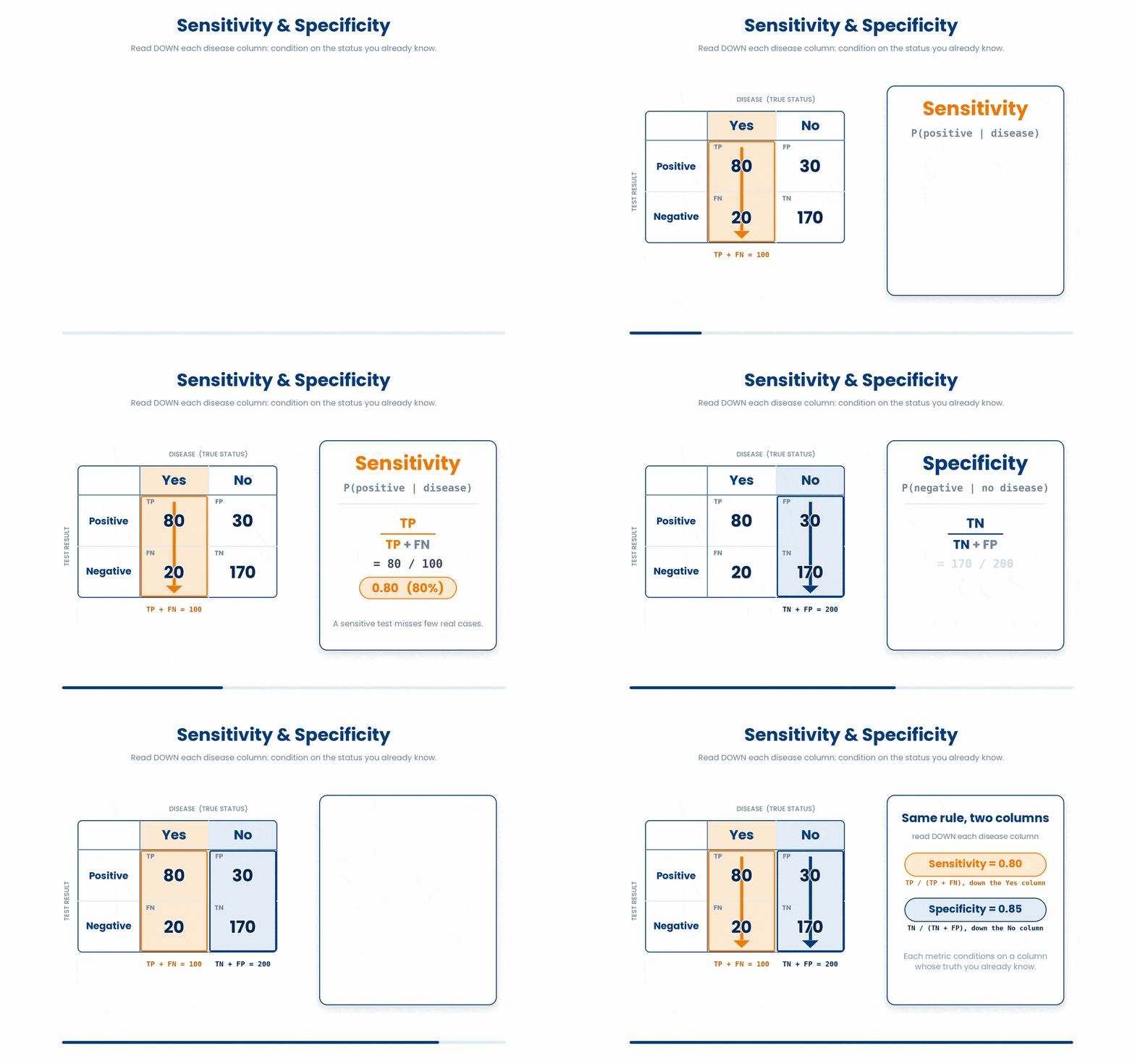
From our table, sensitivity is 90 / (90 + 10), which is 0.90, and specificity is 93 / (93 + 7), which is 0.93. The test catches 90% of real cases and correctly clears 93% of healthy people.

tp <- 90
fp <- 7
fn <- 10
tn <- 93
sensitivity <- tp / (tp + fn)
specificity <- tn / (tn + fp)
c(Sensitivity = sensitivity, Specificity = specificity)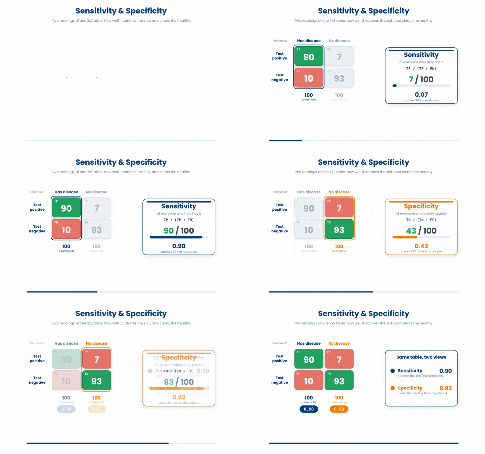

Here is the property that makes these two numbers special: sensitivity and specificity do not change when the disease becomes more or less common. They are fixed characteristics of the test, measured against patients of known status. Move the same test to a clinic with twice the prevalence and the sensitivity stays put.

You have reached the end of the module. Try the same questions again — your answers here, paired with your pre-test answers, are how we measure what the module taught you. Answer every question and confidence rating, then click Submit and see results to view your score.

Here is how your post-test answers compare with your pre-test answers. The pre/post pairing is the most reliable way to see what this module actually taught you.