

1 Before you start
This is not graded, and it does not count towards anything. Answer every question even if you are only guessing — having a go at something before you have been taught it is one of the best ways to remember it afterwards. The lesson ends with another short check, and there you will be shown the correct answer for anything you missed. Choose an option for every question and confidence rating, then click Submit answers.
Which two numbers fully describe a Normal distribution?
A measurement is roughly Normal. About what fraction of values fall within two standard deviations of the mean?
Adult systolic BP is roughly Normal with mean 130 mmHg and SD 10 mmHg. A reading of 165 mmHg is best described as
Hospital length-of-stay has a long right tail. Why is the 68-95-99.7 rule unsafe here?
A patient's fasting glucose is 8.0 mmol/L, where the population mean is 6.0 and the SD is 1.0. What is the z-score?
A ward counts unplanned admissions each night, with no fixed maximum. Which distribution describes this count?
You want the probability that a Normally distributed lab value falls BELOW a patient's reading. Which R function gives this directly?
You need the systolic BP that marks the 95th percentile of a Normal(mean = 120, sd = 15) population. Which call gives it directly?
I can use the 68-95-99.7 rule to judge whether a clinical value is unusual, and I know it only applies when the measurement is roughly Normal.
I can convert a raw measurement to a z-score with (x - mean) / sd and explain why standardising lets me compare values measured on different scales.
I can tell a Binomial count from a Poisson count, and use the d, p, q, and r prefixes to get an exact probability, a tail probability, a percentile, and a simulated sample in R.
2 Introduction
In Part I you combined the chances of separate events — this OR that, this AND that — and met the idea that one event can change the odds of another. But most clinical measurements are not yes/no events. Height, blood pressure, a lab result vary along a continuous scale, and to reason about them you need a shape that describes how the values spread. This part gives you that shape, a way to place any single value on it, and the R functions that turn the whole picture into numbers.
This part of the module covers four foundations, each one feeding the next:
- The Normal distribution — the symmetric bell curve and the 68-95-99.7 rule for spotting an unusual clinical value at a glance.
- z-scores — standardising any measurement to how many standard deviations it sits above or below the mean, so values on different scales become comparable.
- Counts and rates — the Binomial and Poisson distributions named and told apart, for outcomes you count rather than measure.
- The d/p/q/r family — one tidy naming convention that does the work for every distribution, so a tail probability is one call to pnorm away.
By the end of this part you will be able to use the 68-95-99.7 rule to judge whether a clinical value is unusual, convert a raw measurement to a z-score by hand, recognise whether a count is Binomial or Poisson, and ask R directly for a density, a tail probability, a percentile, or a simulated sample with the d/p/q/r prefixes.
Try every snippet in the R Scratchpad on the right. This part needs no data file — you will build small examples with c() and let base R and ggplot2 draw the curves, then let rnorm() simulate patients for you.
3 The Normal distribution and the 68-95-99.7 rule
So far you have combined probabilities of separate events. Many clinical measurements, though, vary along a continuous scale — height, blood pressure, a lab value. To reason about those, you need a shape that describes how the values spread. That shape is the Normal distribution.
The Normal distribution is the symmetric, bell-shaped curve that many biological measurements follow. It is described by two numbers: its mean (where the peak sits) and its standard deviation or SD (how wide the bell is). Most values cluster near the mean, and values get rarer the further out you go.
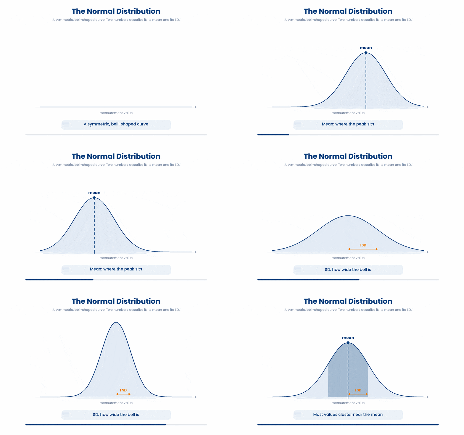
The 68-95-99.7 rule — the empirical rule — tells you how much of the data falls within a few SDs of the mean for any Normal distribution:
- About 68% of values lie within 1 SD of the mean.
- About 95% lie within 2 SDs.
- About 99.7% lie within 3 SDs.
Make it clinical. Suppose adult systolic blood pressure is roughly Normal with a mean of 130 mmHg and an SD of 10 mmHg. Then about 95% of people fall between 110 and 150 mmHg (two SDs each way). A reading of 165 sits beyond three SDs — genuinely unusual, worth a second look.
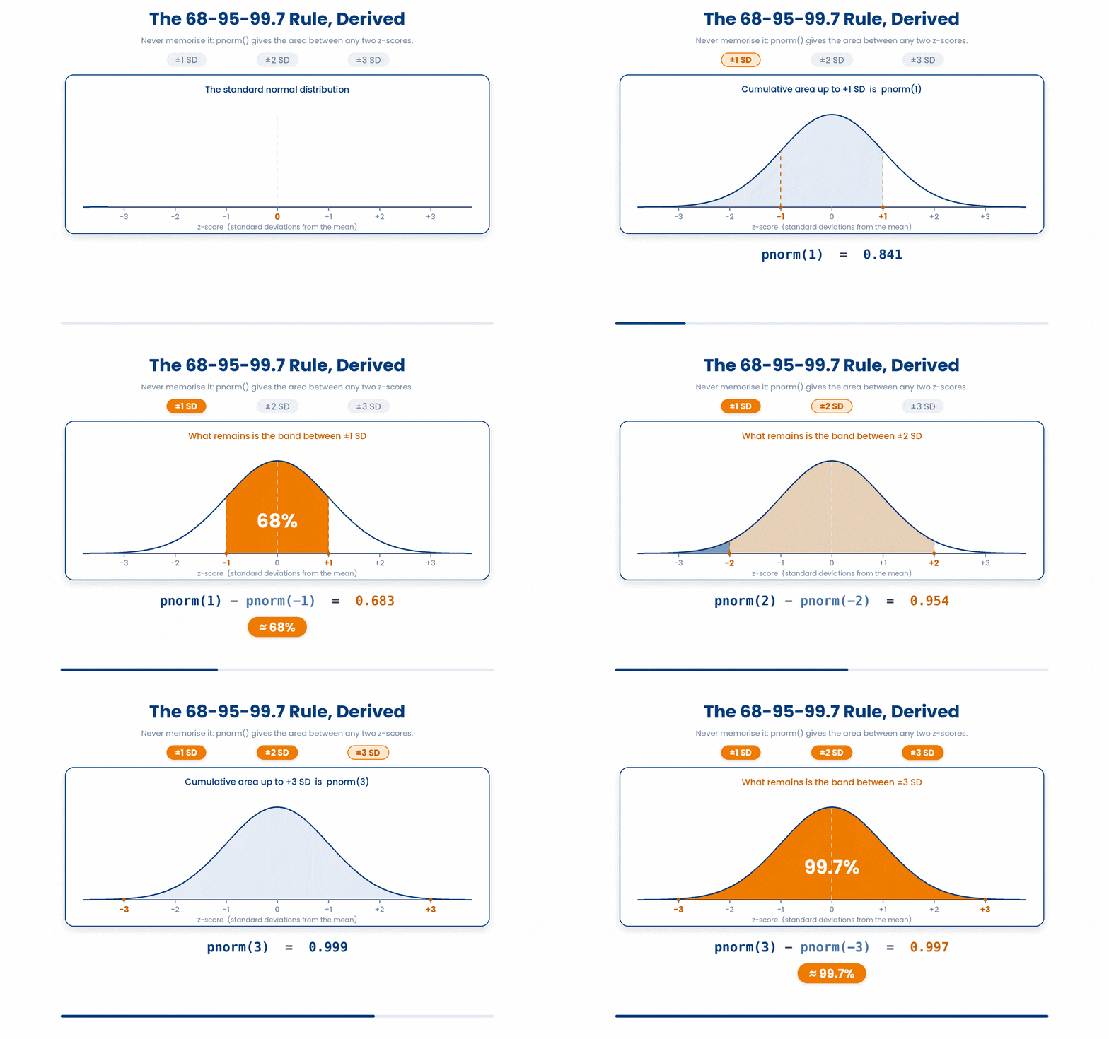
Here is the line that separates a useful rule from a wrong one: the 68-95-99.7 rule only holds when the data are roughly Normal. Applied to a skewed measurement like hospital length-of-stay, which has a long right tail, it will badly mislead you. Always ask whether the bell shape is plausible before you reach for it.
3.1 Sketching the curve in R
Seeing the curve fixes the rule in your memory. Base R draws a function over a range with curve(), and ggplot2 does the same with stat_function(). Pass dnorm — the function that gives the curve's height — and a mean and SD.
Run this to draw the blood-pressure curve. A ggplot must be printed at the top level to appear, so end the pipeline without assigning it to a name.
Try this snippet in the R Scratchpad on the right.
library(ggplot2)
ggplot(data.frame(x = c(100, 160)), aes(x)) +
  stat_function(fun = dnorm, args = list(mean = 130, sd = 10)) +
  labs(x = "Systolic BP (mmHg)", y = "Density")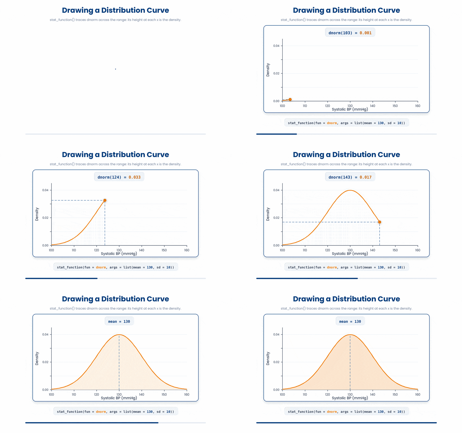
4 z-scores: how many SDs from the mean
The 68-95-99.7 rule tells you what is unusual, but only in whole SDs. To place any single value precisely, you convert it to a z-score. This is the bridge from a raw measurement to a probability.
A z-score restates a measurement as how many standard deviations it lies above or below the mean. The formula is (x - mean) / sd. A z-score of 0 sits exactly at the mean; +2 is two SDs above; -1.5 is one and a half SDs below. The sign tells you the direction, the size tells you how extreme.
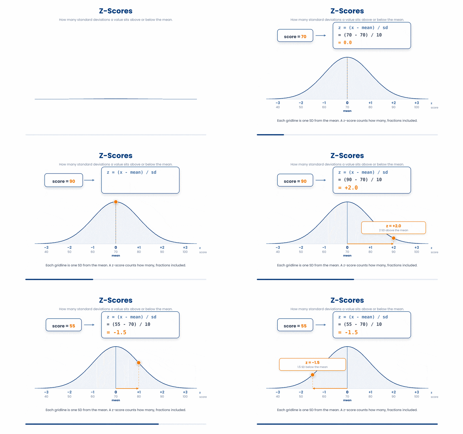
Take a patient with a systolic pressure of 150 mmHg, against a mean of 130 and an SD of 10. Their z-score is (150 - 130) / 10, which is 2. They sit exactly two SDs above the mean — at the edge of the usual range.
Standardising lets you compare measurements on completely different scales. A z-score of +2 is equally unusual whether it came from blood pressure in mmHg or cholesterol in mmol/L. Subtract the mean before you divide — writing x - mean / sd divides only the mean by the SD, because R does the division first. Wrap the subtraction in parentheses.
Try this snippet in the R Scratchpad on the right.
x <- 150
mean_bp <- 130
sd_bp <- 10
z <- (x - mean_bp) / sd_bp
z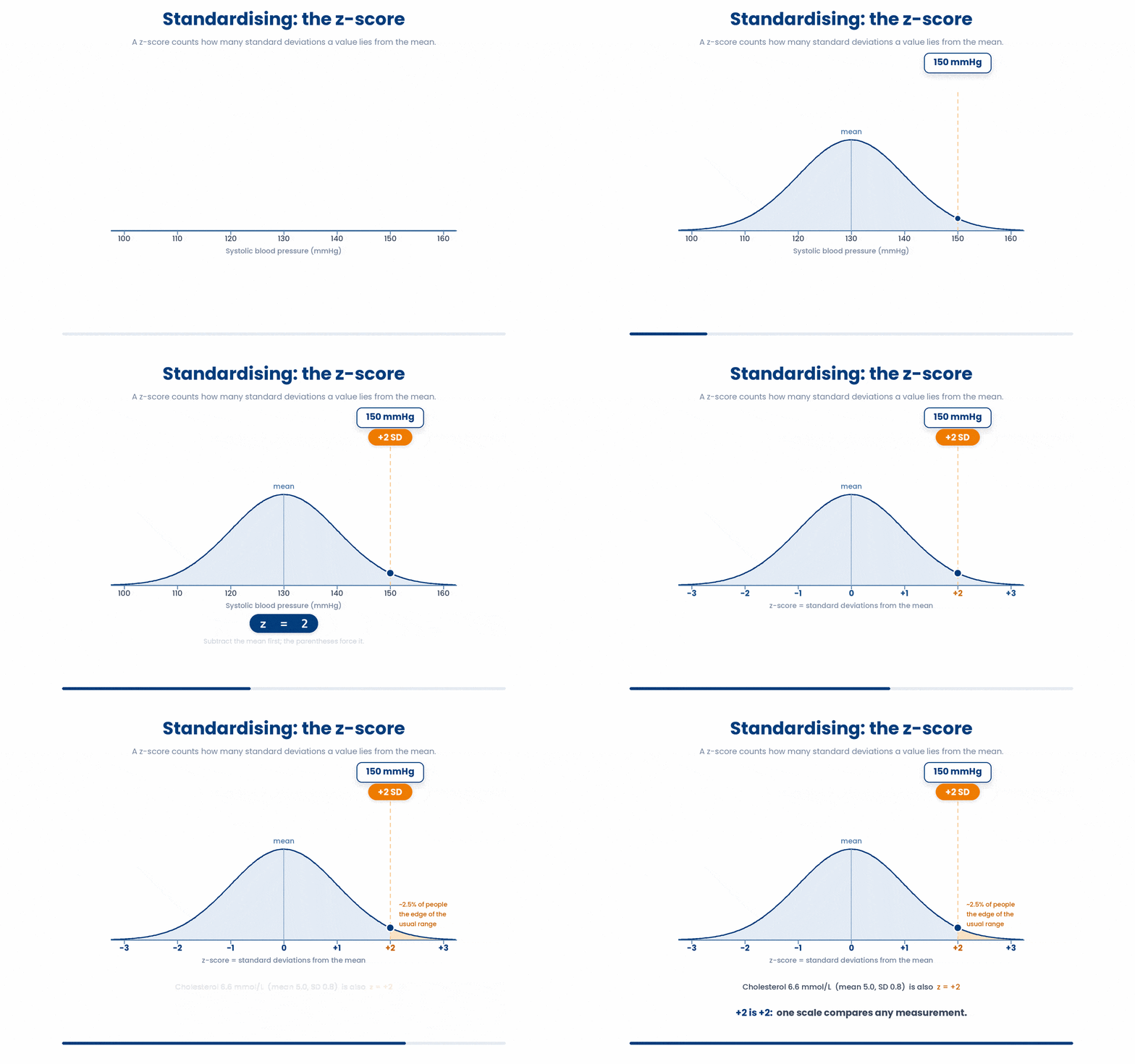
5 Counts, rates, and the d/p/q/r family in R
Not every clinical outcome is a continuous measurement like blood pressure or BMI. Often, you count things: how many patients out of twenty responded to a therapy, or how many admissions arrived overnight. Two named distributions describe these counts perfectly, and one tidy family of R functions handles them all.
5.1 Binomial distribution
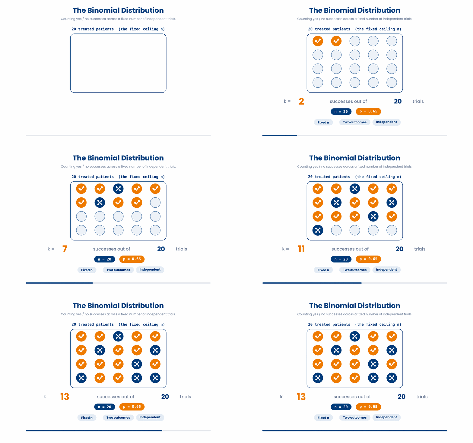
The Binomial distribution describes the count of yes/no successes in a fixed number of independent tries. If you can phrase your outcome as " events out of total trials," you are likely in Binomial territory.
- Clinical Example: The number of patients who respond to a new biologic drug out of 20 treated. The number of successful intubations out of 50 attempts.
- The Key Assumptions: You need a known, fixed ceiling (the 20 patients). Each trial must have only two possible outcomes (success/failure, alive/dead, responded/did not respond). Finally, the trials must be independent—one patient responding shouldn't change the probability of the next patient responding.
- The Parameters: It is defined by (the number of trials) and (the probability of success for each trial).
5.2 Poisson distribution
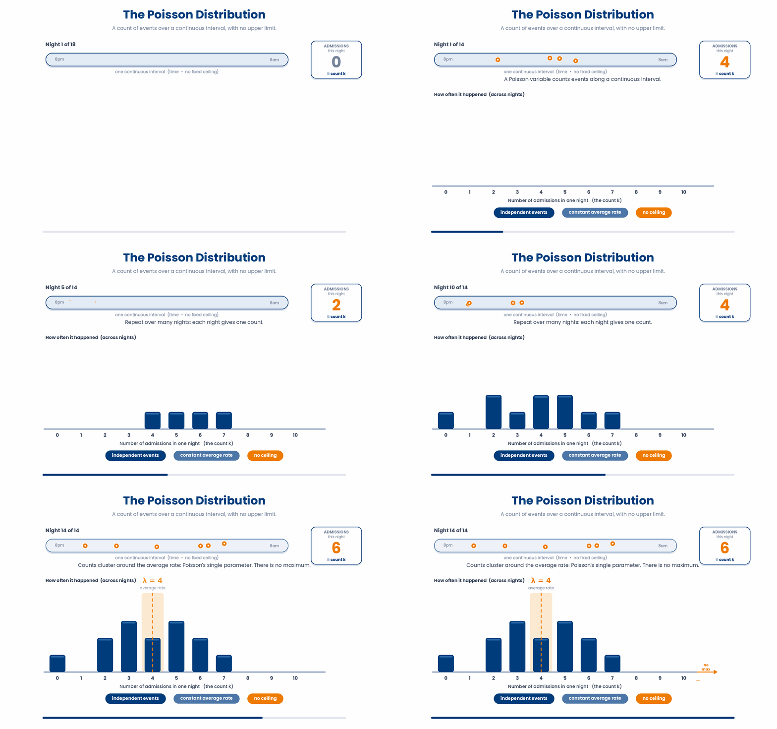
The Poisson distribution describes a count of events over a continuous span of time, space, or volume when there is no fixed ceiling. You cannot count how many times an event did not happen.
- Clinical Example: The number of A&E admissions in one night, the number of asthma exacerbations a patient suffers in a year, or the number of bacterial colonies on an agar plate.
- The Key Assumptions: Events must occur independently of each other. The average rate of events must be constant over the interval you are measuring. Crucially, there is no natural maximum—in theory, an infinite number of patients could walk into A&E, even if it is highly improbable.
- The Parameter: It is defined entirely by a single value, (lambda), which is the average rate or expected number of events in that interval.
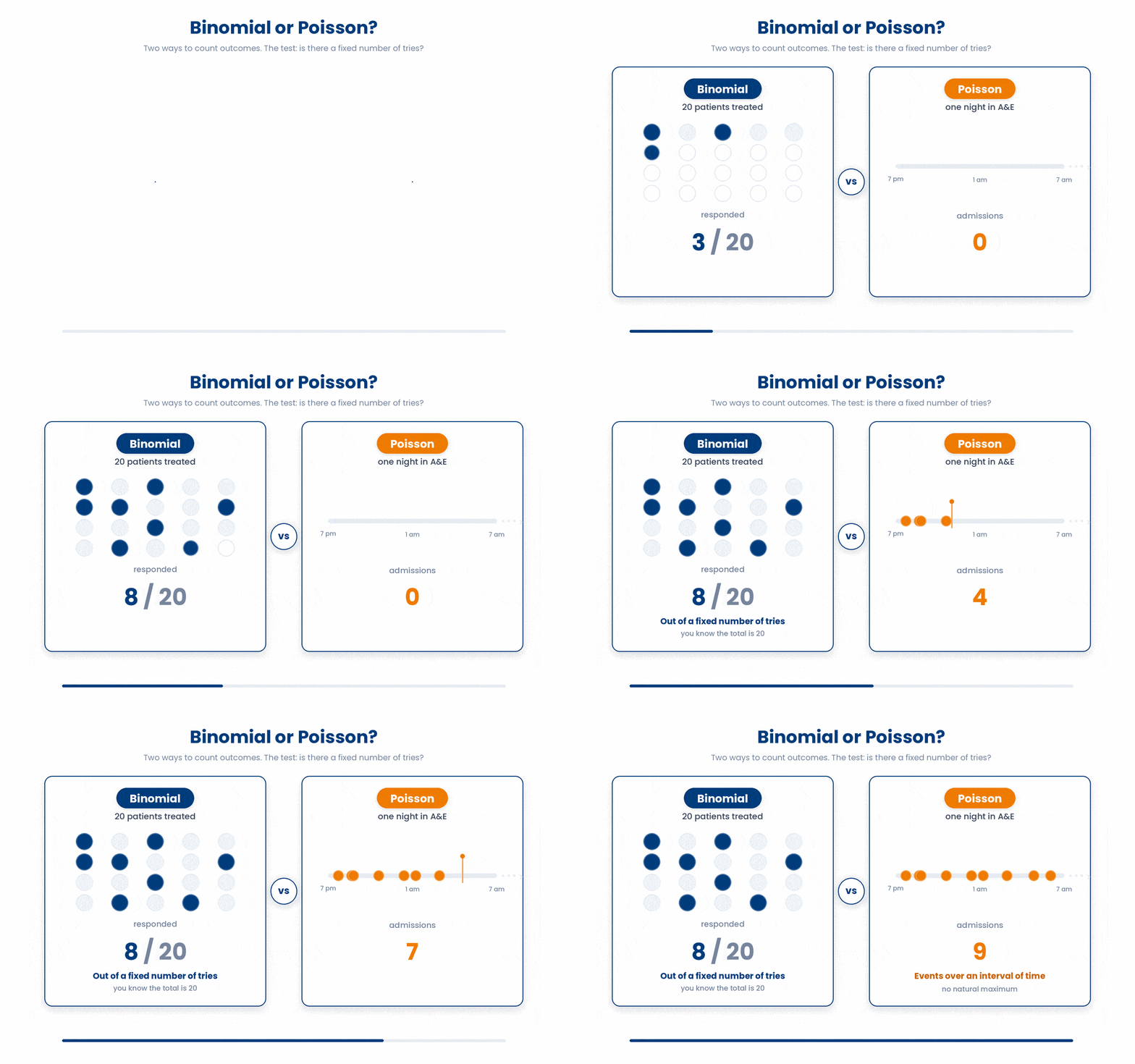
You do not need the formulas. You need to recognise which is which: a count out of a known total of tries is Binomial; a count of events over an interval with no natural maximum is Poisson.
Here is a summary image of when to use binomial or poisson distribution.
5.3 Tidy Family of R Functions
R uses an elegant and consistent naming convention for every distribution function: a single-letter prefix attached to the distribution's short name. For the Normal distribution, the short name is norm. For the count distributions, they are binom and pois.
Learn the four prefixes once, and they work for every distribution you will ever encounter.
1. d for density/exact probability
The d prefix behaves differently depending on whether your data is continuous (like blood pressure) or discrete (like counts).
For a continuous distribution like the Normal (dnorm), this returns the density—the height of the curve at a specific value. It is not a probability, and its value can even exceed 1 for a very narrow curve.
For discrete distributions, the d prefix does return an exact probability. dbinom gives the Binomial probability of an exact count, and dpois gives the Poisson probability of an exact count.
Try this snippet in the R Scratchpad on the right.
# 25 vaccinated patients, each 15% chance of a sore arm. P(exactly 4)?
dbinom(4, size = 25, prob = 0.15)

# A&E sees on average 6 fractures a night. P(exactly 9 tonight)?
dpois(9, lambda = 6)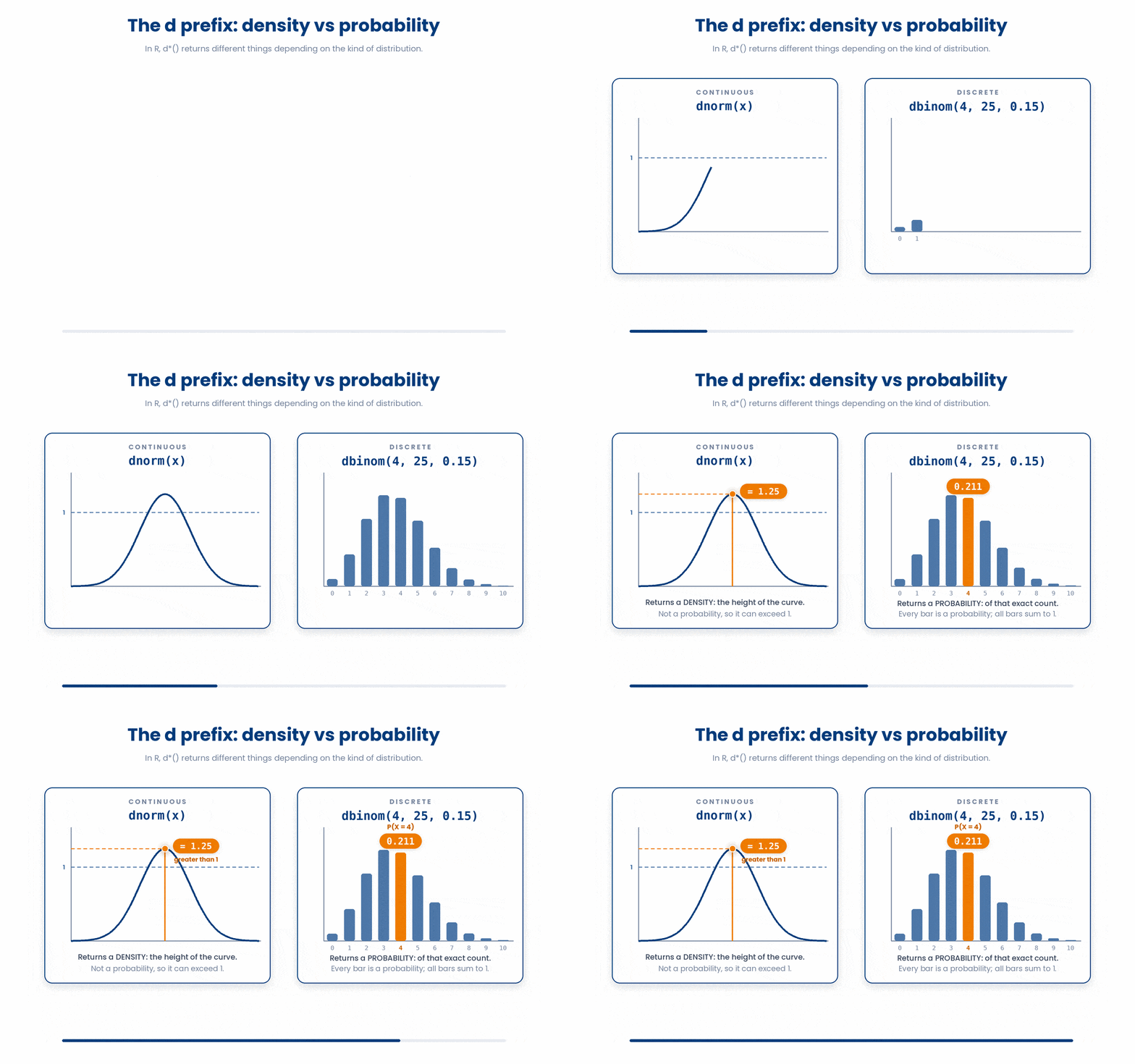
2. p for cumulative probability
Reach for the p prefix whenever a question asks "how likely?" It returns the probability of being at or below a certain value—the area under the curve to its left. At the exact center of a Normal curve, half the area lies to the left, so pnorm(0) returns 0.5.
By default, p functions return the left tail (the probability below a value). To get the chance of being above a value, you need the upper tail. If you forget to specify this, you will get the exact opposite of the answer you wanted.
Try this snippet in the R Scratchpad on the right.
# Systolic BP ~ Normal(mean = 120, sd = 15) mmHg.
# What proportion of patients are above 140 mmHg (hypertension)?
pnorm(140, mean = 120, sd = 15, lower.tail = FALSE)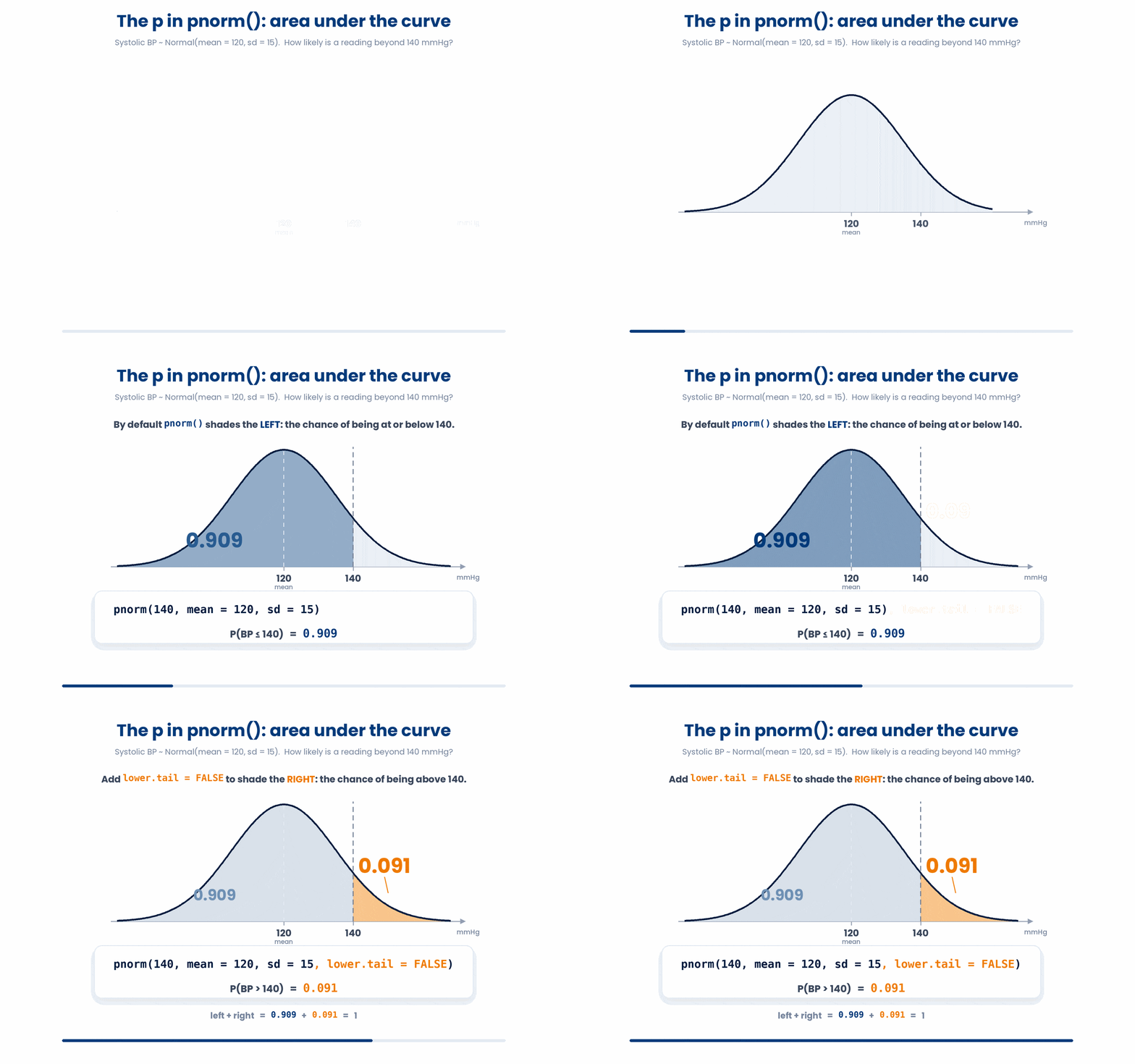
3. q for quantile
The q prefix does the exact opposite of p. It runs in reverse, mapping a probability back to a specific value or z-score.
If you want to know which z-score cuts off the top 2.5% of a Normal distribution, you ask for the 97.5th percentile. This gives you the famous 1.96 multiplier that every 95% confidence interval is built upon.
Try this snippet in the R Scratchpad on the right.
# Systolic BP ~ Normal(mean = 120, sd = 15) mmHg.
# Which BP marks the 95th percentile (top 5% of patients)?
qnorm(0.95, mean = 120, sd = 15)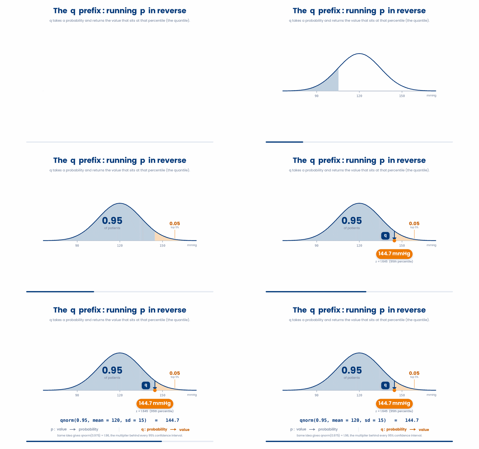
4. qr for quantile
The r prefix generates random, simulated data from the distribution. rnorm(100) will simulate 100 values from a standard Normal distribution, while rbinom or rpois will simulate repeated clinical trials or event counts.
Because you have pnorm, you never actually need to memorize the 68-95-99.7 empirical rule for Normal distributions. You can verify the area between standard deviations yourself by subtracting the left tail from the right tail:
Try this snippet in the R Scratchpad on the right.
# Area between -1 and +1 SD (approx 68%)
pnorm(1) - pnorm(-1)

# Area between -2 and +2 SD (approx 95%)
pnorm(2) - pnorm(-2)

# Area between -3 and +3 SD (approx 99.7%)
pnorm(3) - pnorm(-3)Try this out
Try this snippet in the R Scratchpad on the right.
# Simulate systolic BP for 30 patients: Normal(mean = 120, sd = 15).
bp <- rnorm(30, mean = 120, sd = 15)
round(bp, 1) # the simulated readings
mean(bp) # sample mean: near 120, but not exactly
sum(bp > 140)  # how many would be flagged hypertensive?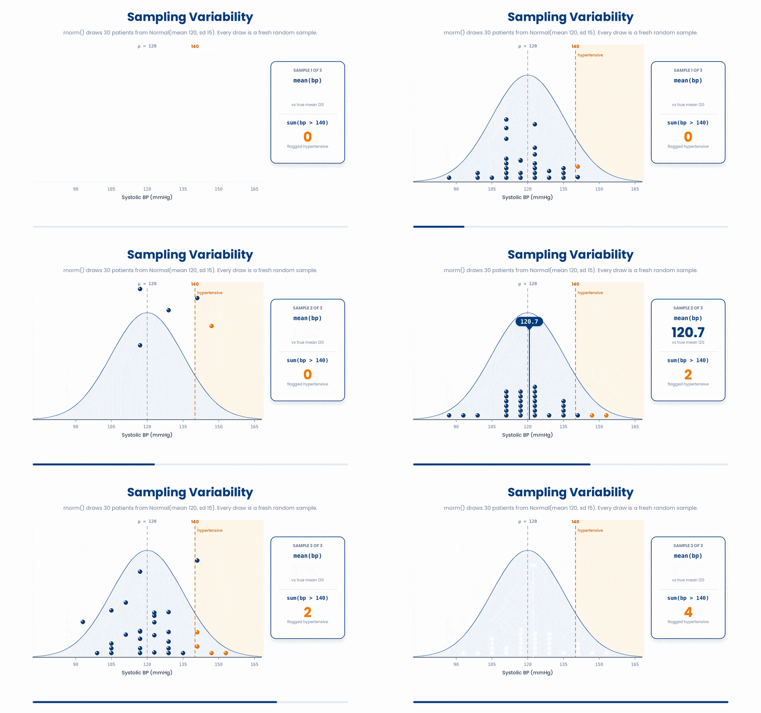
6 Put it together
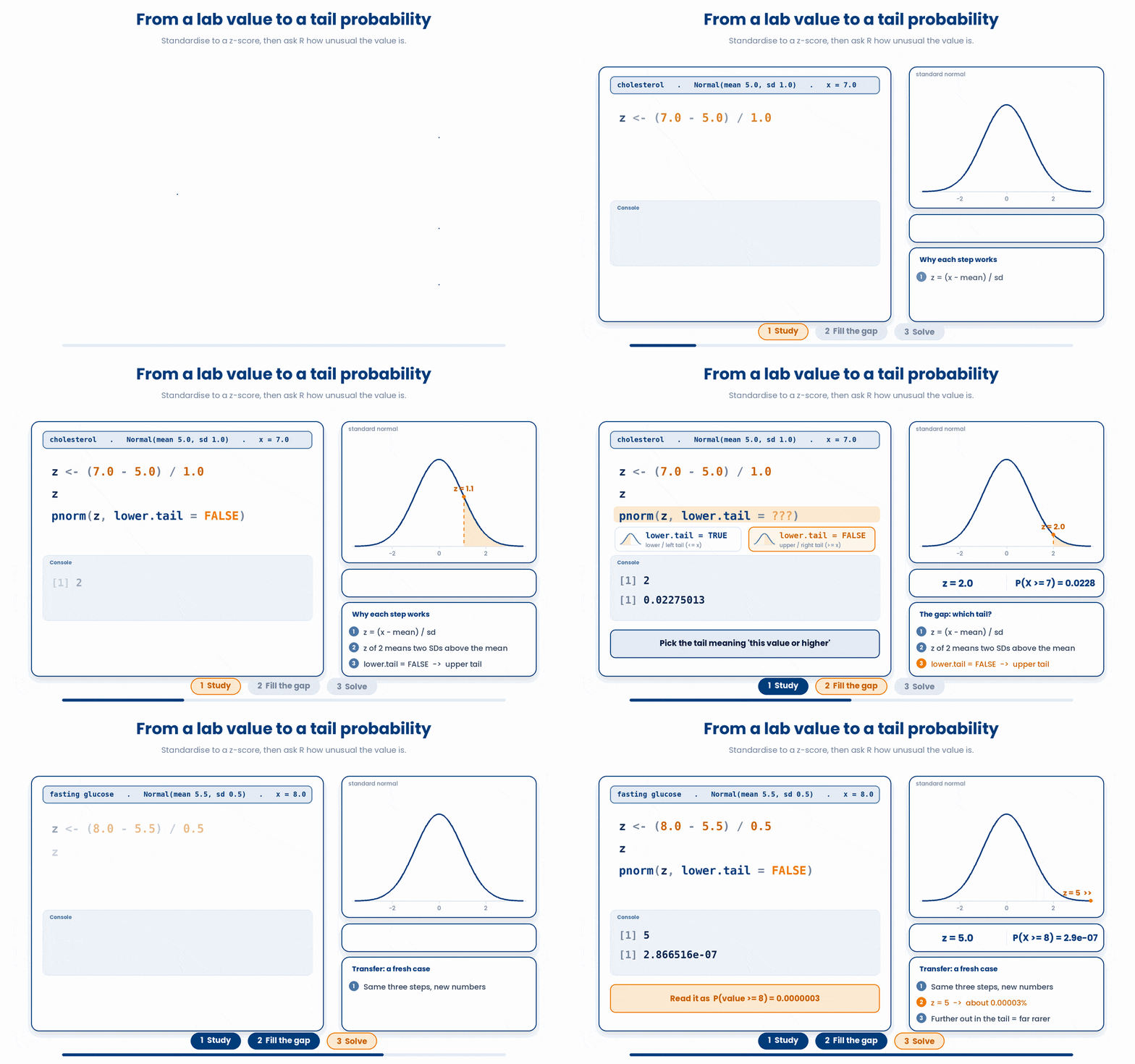
Now you will run the full chain: take a raw clinical measurement, standardise it to a z-score, and ask R for the tail probability that tells you how unusual it is. The worked example fades its support — study the full solution, then fill the gap, then solve a fresh one.
Work through this example in three stages. You unlock each stage only after the tutor confirms the previous one. Each stage removes more of the scaffolding — by the end you are writing it yourself.
Problem: Total cholesterol in a population is roughly Normal with mean 5.0 mmol/L and SD 1.0 mmol/L. A patient measures 7.0 mmol/L. Convert that to a z-score, then find the probability of a value this high or higher.
z <- (7.0 - 5.0) / 1.0
z
pnorm(z, lower.tail = FALSE)- Compute the z-score with (x - mean) / sd, wrapping the subtraction in parentheses
- A z of 2 means the patient is two SDs above the mean
- pnorm with lower.tail = FALSE gives the upper tail — the chance of being this high or higher
The same solution with key parts replaced by ???.
Fill in every ??? so the code matches the reference,
then ask the tutor to check it.
Your turn: Now do the same for a patient whose fasting glucose is 8.0 mmol/L, where the population mean is 5.5 mmol/L and the SD is 0.5 mmol/L. Report the z-score and the probability of a value this high or higher.
7 Check your understanding
You have reached the end of the module. Try the same questions again — your answers here, paired with your pre-test answers, are how we measure what the module taught you. Answer every question and confidence rating, then click Submit and see results to view your score.
Which two numbers fully describe a Normal distribution?
A measurement is roughly Normal. About what fraction of values fall within two standard deviations of the mean?
Adult systolic BP is roughly Normal with mean 130 mmHg and SD 10 mmHg. A reading of 165 mmHg is best described as
Hospital length-of-stay has a long right tail. Why is the 68-95-99.7 rule unsafe here?
A patient's fasting glucose is 8.0 mmol/L, where the population mean is 6.0 and the SD is 1.0. What is the z-score?
A ward counts unplanned admissions each night, with no fixed maximum. Which distribution describes this count?
You want the probability that a Normally distributed lab value falls BELOW a patient's reading. Which R function gives this directly?
You need the systolic BP that marks the 95th percentile of a Normal(mean = 120, sd = 15) population. Which call gives it directly?
I can use the 68-95-99.7 rule to judge whether a clinical value is unusual, and I know it only applies when the measurement is roughly Normal.
I can convert a raw measurement to a z-score with (x - mean) / sd and explain why standardising lets me compare values measured on different scales.
I can tell a Binomial count from a Poisson count, and use the d, p, q, and r prefixes to get an exact probability, a tail probability, a percentile, and a simulated sample in R.
8 Your results
Here is how your post-test answers compare with your pre-test answers. The pre/post pairing is the most reliable way to see what this module actually taught you.
Submit the post-test to see your results.
What is the one thing from this module that is still unclear to you?