

1 Before you start
This is not graded, and it does not count towards anything. Answer every question even if you are only guessing — having a go at something before you have been taught it is one of the best ways to remember it afterwards. The lesson ends with another short check, and there you will be shown the correct answer for anything you missed. Choose an option for every question and confidence rating, then click Submit answers.
A categorical variable such as treatment arm has no mean. How should you summarise it?
Which line gives a count and proportion for each category of the sex column in a data frame called patients?
After tabyl(smoker), which adorn helper turns the raw proportions into readable percentages?
You want a table of sex down the rows and smoking status across the columns. Which call builds that cross-tabulation?
Your call mean(hba1c) returns NA because the column has one missing value. What is R telling you?
Your call mean(hba1c) returns NA because the column has one missing value. Which line reports the mean of the values you do have?
Which expression reports how many values in the hba1c column are missing?
You set na.rm = TRUE and report the median. Why should you also report n missing beside it?
I can summarise a categorical variable with tabyl() as counts and proportions, and format the proportions as readable percentages.
I can cross-tabulate two categorical variables with tabyl() and add totals and row percentages to compare the groups.
I can explain why mean() returns NA when a value is missing, fix it with na.rm = TRUE, and count and report the missing values with sum(is.na(column)) so my summary stays honest.
2 Introduction
In Part I you summarised a numeric column with the right centre-and-spread pair — mean (SD) for a symmetric variable, median (IQR) for a skewed one. But many of the columns your reader cares about are not numbers at all: sex, treatment arm, smoking status. And every real clinical dataset has holes — a patient skips a blood test and the cell is blank. This part gives you the tools for both: summarising categories, and summarising honestly when values are missing.
This part of the module covers two skills:
- Categorical summaries — counts and proportions for each group with tabyl(), and a cross-tabulation of two categorical variables to ask whether they are related.
- Honest summaries — handling missing values with na.rm = TRUE, and counting and reporting how many patients you dropped so the holes never hide.
By the end of this part you will be able to tabulate a categorical variable as counts and proportions, cross-tabulate two categories and add totals and row percentages, explain why mean() returns NA when a value is missing, fix it with na.rm = TRUE, and count missing values with sum(is.na(column)) so you never silently hide missing data.
Try every snippet in the R Scratchpad on the right. The datasets patients.csv and diabetes_clinic.csv are already loaded — the first for the categorical tables, the second (which contains missing HbA1c values) for the honest-summary examples.
3 Summarising categorical variables
Location and spread describe numbers. A categorical variable — sex, treatment arm, smoking status — has no average. You summarise it with a count (how many patients in each group) and a proportion (what fraction of the total each group is). Counts and proportions are to categories what the mean and SD are to numbers.
The cleanest way to build a count table is tabyl() from the janitor package. Give it a data frame and a column, and it returns the count and the proportion in one tidy table.
Try this snippet in the R Scratchpad on the right.
library(readr)
library(janitor)
patients <- read_csv("patients.csv")
patients |> tabyl(sex)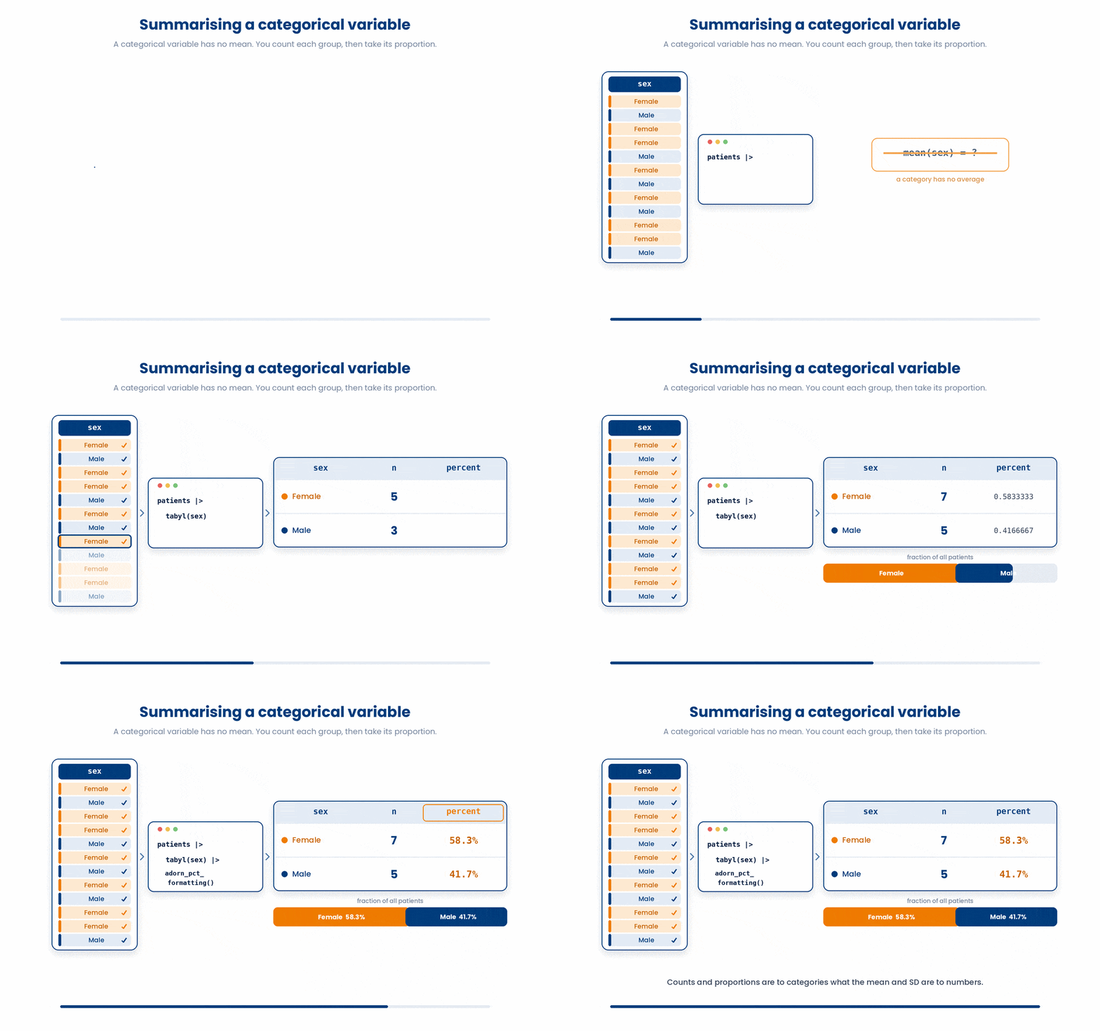
The adorn_*() helpers then dress it up — adorn_pct_formatting() turns the raw proportions into readable percentages.
Try this snippet in the R Scratchpad on the right.
library(readr)
patients <- read_csv("patients.csv")
library(janitor)
patients |>
  tabyl(smoker) |>
  adorn_pct_formatting()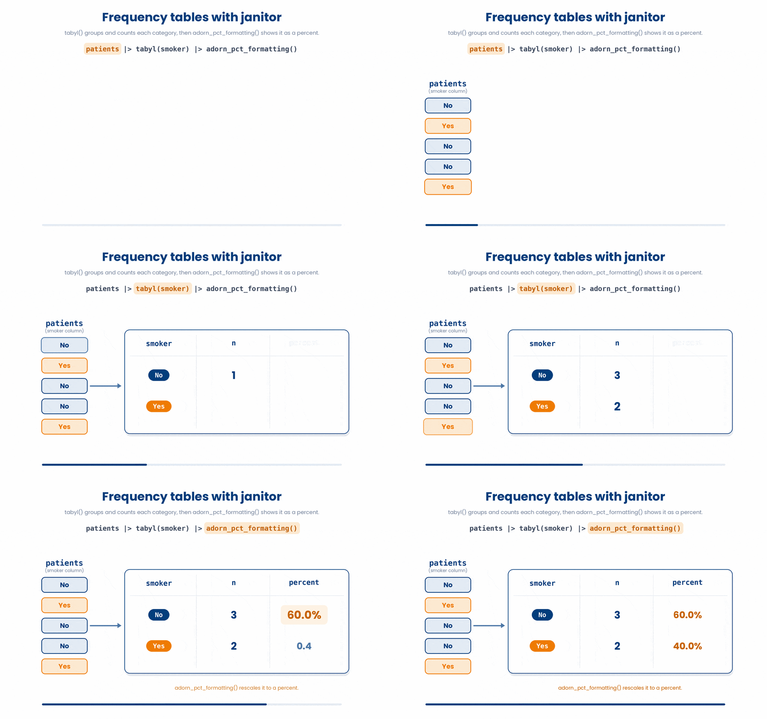
3.1 Cross-tabulating two categories
To ask whether two categories are related — does smoking differ by sex? — you build a cross-tabulation: a table with one variable down the rows and the other across the columns, counting patients in each cell. Pass tabyl() two column names to get one.
The adorn_*() helpers add the finishing touches a reader expects: adorn_totals() adds row and column totals, and adorn_percentages() converts the counts to proportions within each row.
Try this snippet in the R Scratchpad on the right.
library(readr)
patients <- read_csv("patients.csv")
library(janitor)
patients |>
  tabyl(sex, smoker) |>
  adorn_totals(where = "row")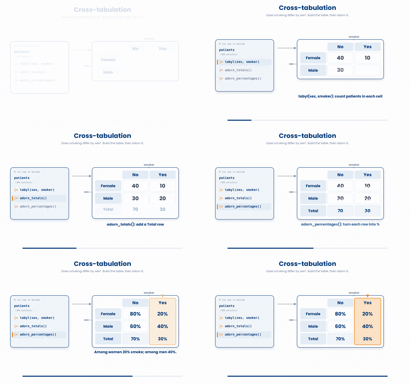
4 Honest summaries: handling missing values
Real clinical data has holes. A patient skips a blood test and that HbA1c cell is NA — R's marker for a missing value, carried over from Module 1. How you treat those holes decides whether your summary is honest.
By default, R is cautious. If even one value in a column is NA, mean() and sd() return NA, not a number. R is telling you: I cannot average values I do not have. This is a feature, not a bug — it stops a silent wrong answer.
To summarise the values you do have, add the argument na.rm = TRUE — read it as "remove the NAs first". Then mean() averages the non-missing values. The same argument works for sd(), median(), IQR(), and friends.
Try this snippet in the R Scratchpad on the right.
median(c(5, 7, NA, 9), na.rm = TRUE)
The first trap is forgetting na.rm = TRUE, so your summary silently returns NA and you report a blank where a number belonged. If a summary comes back as NA, suspect a missing value and add na.rm = TRUE.
The code below is broken. Type a fixed version into the editor, then click Run & check. Success means your code runs without errors. Use Show hint only if you get stuck.
mean(c(7.2, 8.1, NA, 9.4))- Add na.rm = TRUE to average the values you have: mean(c(7.2, 8.1, NA, 9.4), na.rm = TRUE) ★
- Remove the NA by hand: mean(c(7.2, 8.1, 9.4))
- Replace NA with 0: mean(c(7.2, 8.1, 0, 9.4))

The second trap is quieter and worse: dropping incomplete rows without reporting how many you lost. Setting na.rm = TRUE hides the holes; an honest summary states them. Always count the missing values and report n missing alongside your centre and spread.
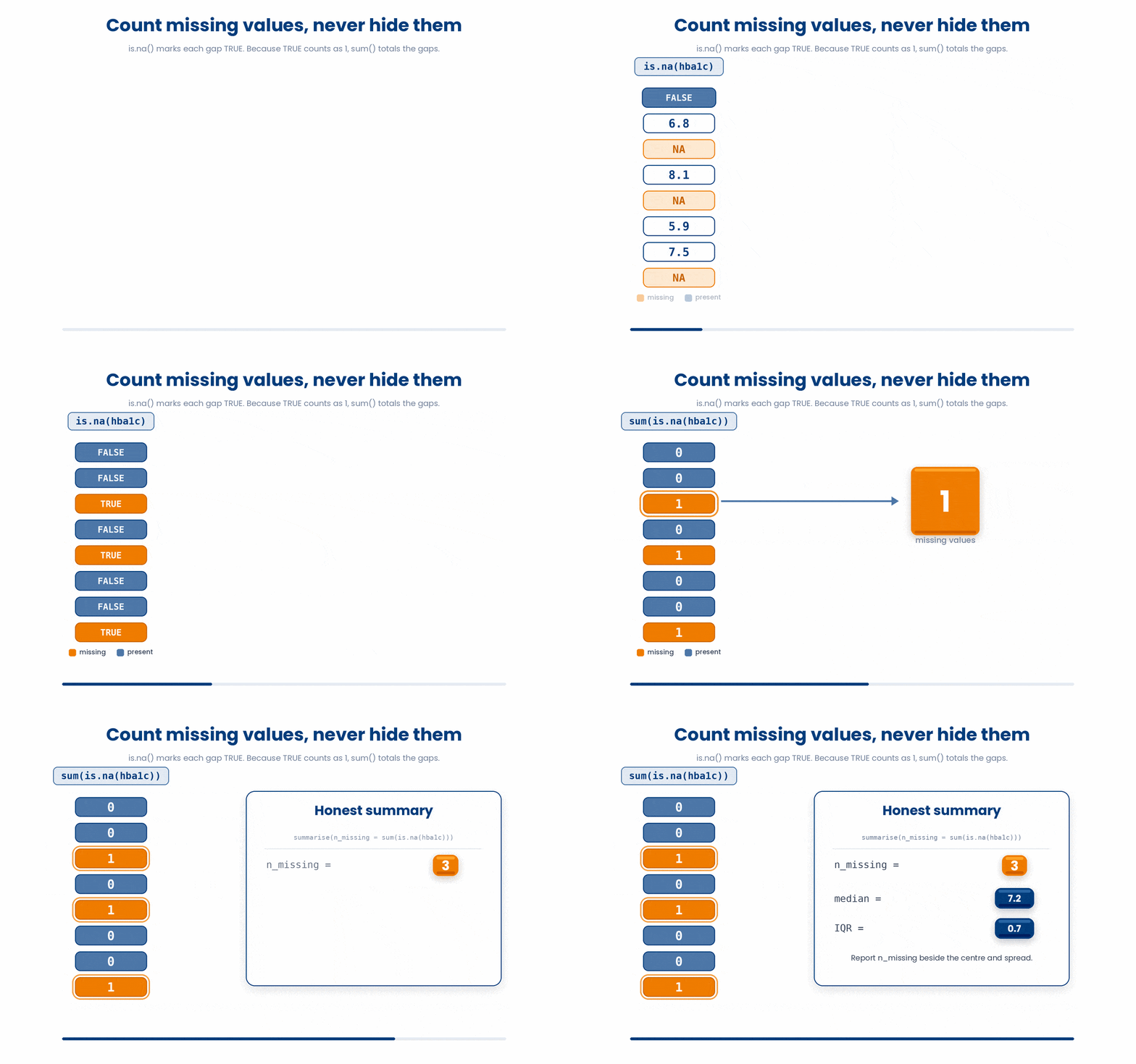
Count missing values by combining two functions: is.na() marks each value TRUE if it is missing, and sum() adds up those TRUEs (because R treats TRUE as 1). So sum(is.na(column)) is the number of missing values.
Try this snippet in the R Scratchpad on the right.
library(readr)
library(dplyr)
clinic <- read_csv("diabetes_clinic.csv")
clinic |>
  summarise(
    n_missing = sum(is.na(hba1c)),
    median_hba1c = median(hba1c, na.rm = TRUE),
    iqr_hba1c = IQR(hba1c, na.rm = TRUE)
  )
5 Put it together
Let’s try this Parsons problem for practice
This Parsons problem gives you the right lines in the wrong order, plus a few lines that do not belong. Drag the correct lines into order and leave the wrong ones in the bank.
All the lines you need are in the Line bank on the left — some may be distractors you should leave behind. Drag the lines you need into the Your solution column on the right, in the correct order, then click Check.
Task: Read the clinic file, then in one summarise() report the number of missing HbA1c values, the median, and the IQR — all missing-aware.
clinic <- read_csv("diabetes_clinic.csv")med = median(hba1c, na.rm = TRUE),iqr = IQR(hba1c, na.rm = TRUE)clinic |> mean(hba1c, na.rm = TRUE)summarise(library(dplyr)clinic |> summarise(med = median(hba1c))clinic |>n_missing = sum(is.na(hba1c)),n_missing <- sum(NA))
- Drop lines here, in order.
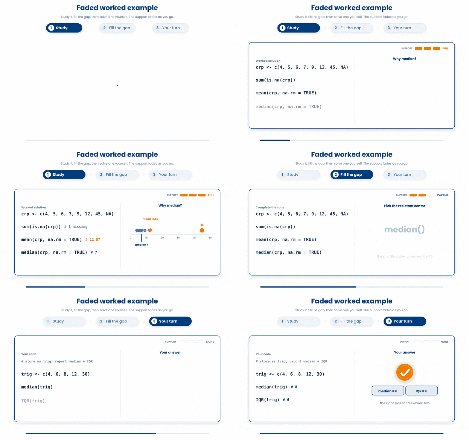
The worked example below fades the support as you go: first you study a full solution, then you fill the gap, then you solve a fresh one on your own. It walks through the whole decision — check for missing values, compare mean and median, and report the right pair.
Work through this example in three stages. You unlock each stage only after the tutor confirms the previous one. Each stage removes more of the scaffolding — by the end you are writing it yourself.
Problem: You have eight CRP results (mg/L), one of them missing: 4, 5, 6, 7, 9, 12, 45, and an NA. Count the missing value, then compare the mean and median to decide which centre to report.
crp <- c(4, 5, 6, 7, 9, 12, 45, NA)
sum(is.na(crp))
mean(crp, na.rm = TRUE)
median(crp, na.rm = TRUE)- sum(is.na(crp)) counts the missing values so you can report n missing
- mean(crp, na.rm = TRUE) averages the seven values you have
- median(crp, na.rm = TRUE) finds the middle value, resistant to the high 45
- the mean lands well above the median, so this lab is right-skewed — report median (IQR)
The same solution with key parts replaced by ???.
Fill in every ??? so the code matches the reference,
then ask the tutor to check it.
Your turn: Now do the same for five triglyceride results: 4, 6, 8, 12, 30 (none missing). Store them in an object called trig, then report the median and the IQR — the right pair for a skewed lab.
6 Check your understanding
You have reached the end of the module. Try the same questions again — your answers here, paired with your pre-test answers, are how we measure what the module taught you. Answer every question and confidence rating, then click Submit and see results to view your score.
A categorical variable such as treatment arm has no mean. How should you summarise it?
Which line gives a count and proportion for each category of the sex column in a data frame called patients?
After tabyl(smoker), which adorn helper turns the raw proportions into readable percentages?
You want a table of sex down the rows and smoking status across the columns. Which call builds that cross-tabulation?
Your call mean(hba1c) returns NA because the column has one missing value. What is R telling you?
Your call mean(hba1c) returns NA because the column has one missing value. Which line reports the mean of the values you do have?
Which expression reports how many values in the hba1c column are missing?
You set na.rm = TRUE and report the median. Why should you also report n missing beside it?
I can summarise a categorical variable with tabyl() as counts and proportions, and format the proportions as readable percentages.
I can cross-tabulate two categorical variables with tabyl() and add totals and row percentages to compare the groups.
I can explain why mean() returns NA when a value is missing, fix it with na.rm = TRUE, and count and report the missing values with sum(is.na(column)) so my summary stays honest.
7 Your results
Here is how your post-test answers compare with your pre-test answers. The pre/post pairing is the most reliable way to see what this module actually taught you.
Submit the post-test to see your results.
What is the one thing from this module that is still unclear to you?