

1 Before you start
This is not graded, and it does not count towards anything. Answer every question even if you are only guessing — having a go at something before you have been taught it is one of the best ways to remember it afterwards. The lesson ends with another short check, and there you will be shown the correct answer for anything you missed. Choose an option for every question and confidence rating, then click Submit answers.
You have a wide DataFrame with columns patient_id, v1, v2, v3 (weights at three visits). Which call turns it into long form with one row per (patient, visit, weight)?
You have a long DataFrame with columns patient_id, timepoint, weight. Which call turns it into wide form — one row per patient, one column per timepoint?
pd.crosstab(df["clinic"], df["sex"]) returns what?
You merge a one-row-per-patient demographics table with a multiple-rows-per-patient labs table using an inner join on patient_id. How many rows does the result have?
You want to keep EVERY row of the demographics table, attaching lab values where a patient has them and NaN where they do not. Which how= do you pass to pd.merge?
pd.get_dummies(df, columns=["clinic"]) does what to the DataFrame?
What is the role of the round brackets in a chained pandas pipeline like (df.pipe(...).merge(...).assign(...))?
df.to_numpy() on a DataFrame of numeric columns returns what?
I can pivot a long-form DataFrame to wide form and melt a wide-form DataFrame to long form.
I can merge two tables on a key column and pick the right join type (inner, left, full outer) for the question I am asking.
I can write a small chained pipeline that joins two tables, one-hot encodes the categorical columns, and bridges into NumPy with .to_numpy().
2 Introduction
Parts I and II covered everything you do with a single DataFrame — reading it in, looking at it, filtering it, cleaning it. Part III is about working across DataFrames and getting your data out the other end. You reshape the table into the form your next tool expects, you combine multiple tables that hold different facts about the same people, you encode categories into numbers, you wrap the whole pipeline into one fluent expression, and finally you hand the result off to NumPy or to disk.
This is the third and final part on pandas. By the end of it you can take two messy CSVs and produce a clean numeric feature matrix in one chained pipeline.
This part covers six tools:
- Reshaping data with pivot and melt — moving between wide form (one column per measurement) and long form (one row per measurement).
- Two-way categorical tables with pd.crosstab — counts in every combination of two categories.
- Joining data — combining two tables with merge, choosing inner, left, or full outer.
- One-hot encoding with pd.get_dummies — turning category labels into 0/1 columns.
- Building processing pipelines with method chaining — writing the whole analysis as one fluent expression that reads top-to-bottom.
- From pandas to NumPy and back — the bridge into the rest of the scientific-Python stack.
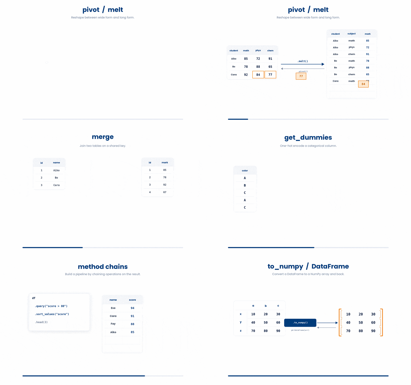
Try every snippet in the Python Scratchpad on the right. By the end of this part you will take two patient tables, join them, encode the categorical columns, chain it all into one pipeline, and convert the result into a NumPy feature matrix.
3 Reshaping data (pivot and melt; wide to long)
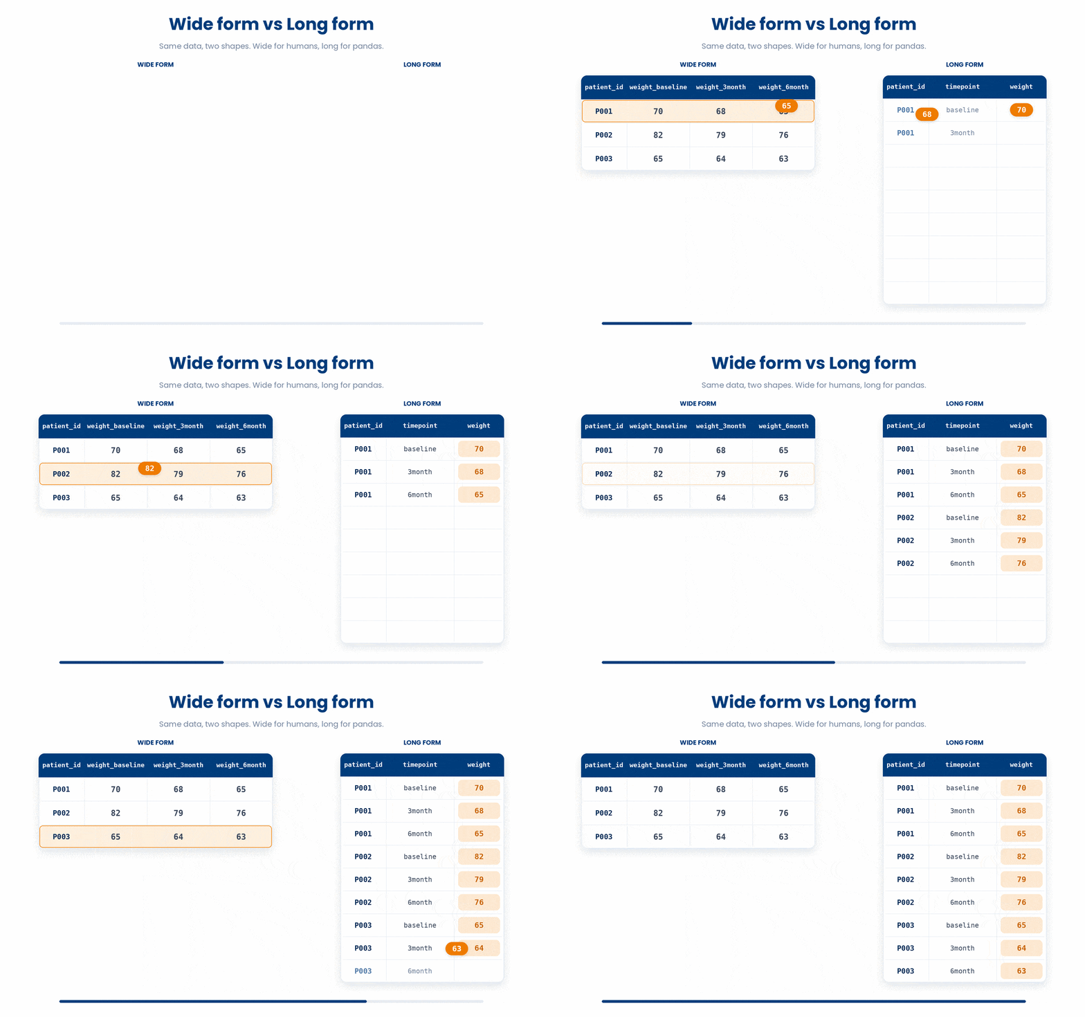
The same information can sit in two very different shapes. In wide form, every measurement type gets its own column (patient_id, weight_baseline, weight_3month, weight_6month), and each row is a single patient. In long form, every measurement is its own row (patient_id, timepoint, weight), and each patient has one row per timepoint. Humans usually find wide form easier to read; pandas almost always finds long form easier to work with. Reshaping moves between the two.
3.1 Wide to long form
Going from wide to long uses pd.melt. You tell it which columns to keep as identifiers (id_vars) and which columns to stack into a single new column (value_vars). The names of the stacked columns become entries in a new "variable" column; their values become entries in a new "value" column. You name both.
Try this snippet in the Python Scratchpad on the right.
import pandas as pd

wide = pd.DataFrame({
    "patient_id": ["P001", "P002"],
    "weight_baseline": [72, 80],
    "weight_3month": [70, 78],
    "weight_6month": [69, 77],
})
long = pd.melt(
    wide,
    id_vars=["patient_id"],
    value_vars=["weight_baseline", "weight_3month", "weight_6month"],
    var_name="timepoint",
    value_name="weight",
)
print(long)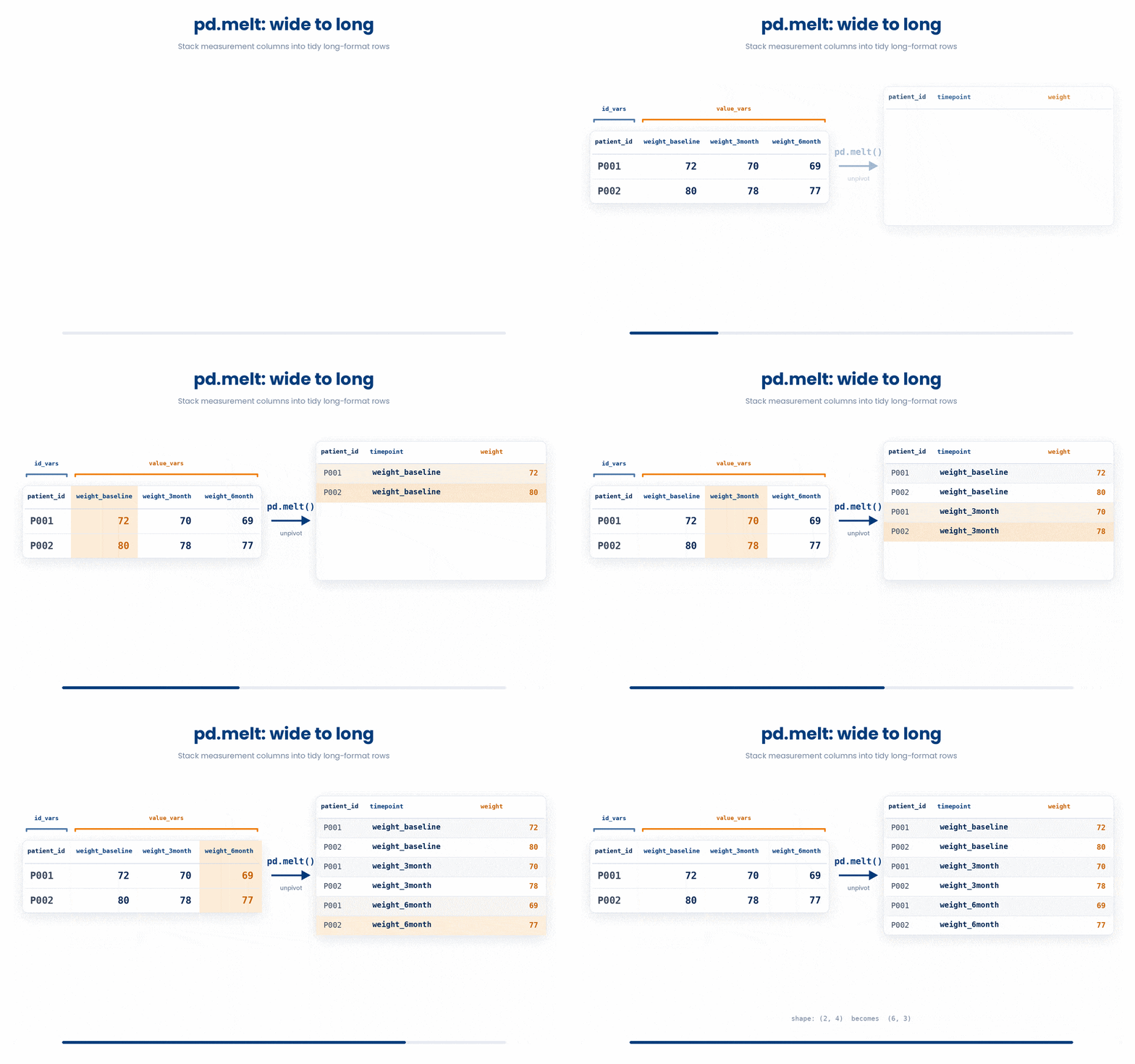
Long form is the natural shape for almost every pandas operation. groupby works on it. Filtering on timepoint is a single boolean expression. Plotting weight against timepoint with a line per patient is one matplotlib call. The wide form looked friendlier to a human eye but did not let you do any of those things.
3.2 Long to wide form
Going from long to wide uses df.pivot. Tell it which column should become the rows (index), which column should become the new columns, and which column holds the values that fill the cells.
Try this snippet in the Python Scratchpad on the right.
import pandas as pd

long = pd.DataFrame({
    "patient_id": ["P001", "P001", "P002", "P002"],
    "timepoint": ["baseline", "3month", "baseline", "3month"],
    "weight": [72, 70, 80, 78],
})
wide = long.pivot(index="patient_id", columns="timepoint", values="weight")
print(wide)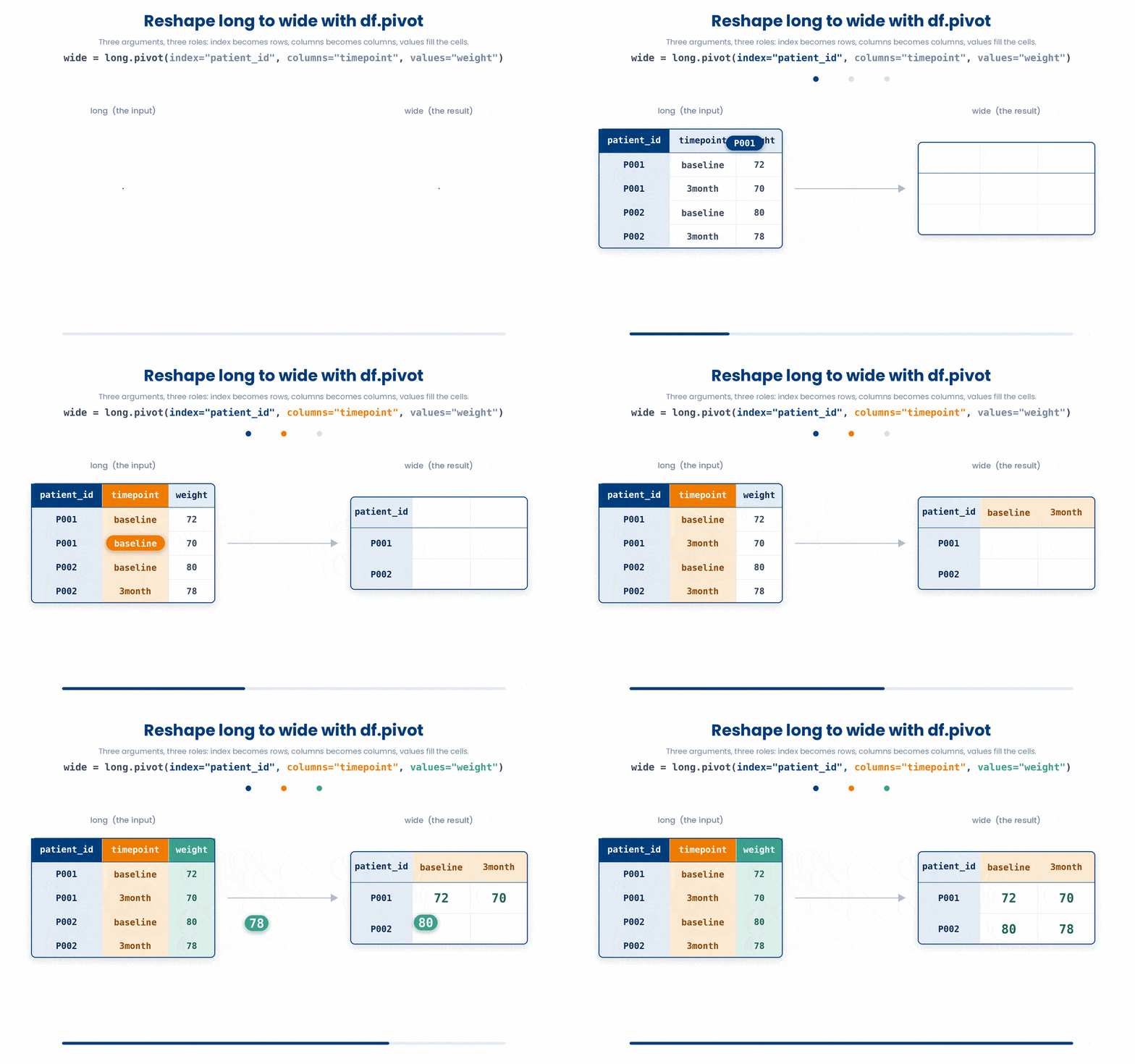
If the same patient_id and timepoint pair shows up more than once in your long data — two readings on the same day, perhaps — plain pivot raises an error because it does not know which value to use. The fix is df.pivot_table, which is the same idea but with an aggfunc argument that says how to combine duplicates. The default aggfunc is mean, but you can pass "median", "max", "first", or any function you want.
4 Two-way categorical tables with pd.crosstab
value_counts summarises one column. To cross-tabulate two - how many patients fall into each combination of clinic and sex - use pd.crosstab. It returns a DataFrame with one column per category on one axis and one row per category on the other.
Try this snippet in the Python Scratchpad on the right.
import pandas as pd

df = pd.DataFrame({
    "clinic": ["A", "A", "B", "B", "C", "C"],
    "sex": ["F", "M", "F", "F", "M", "F"],
})
print(pd.crosstab(df["clinic"], df["sex"]))
5 Joining data (inner, left, full outer)
Different tables hold different facts about the same people. A demographics table has patient_id, age, sex, ethnicity. A lab results table has patient_id, glucose, cholesterol, blood pressure.
To answer a question that crosses both ("what is mean cholesterol by age band?"), you need them combined into one DataFrame, matched up by their shared patient_id. That operation is called a join, and the pandas function is pd.merge.
5.1 Inner join
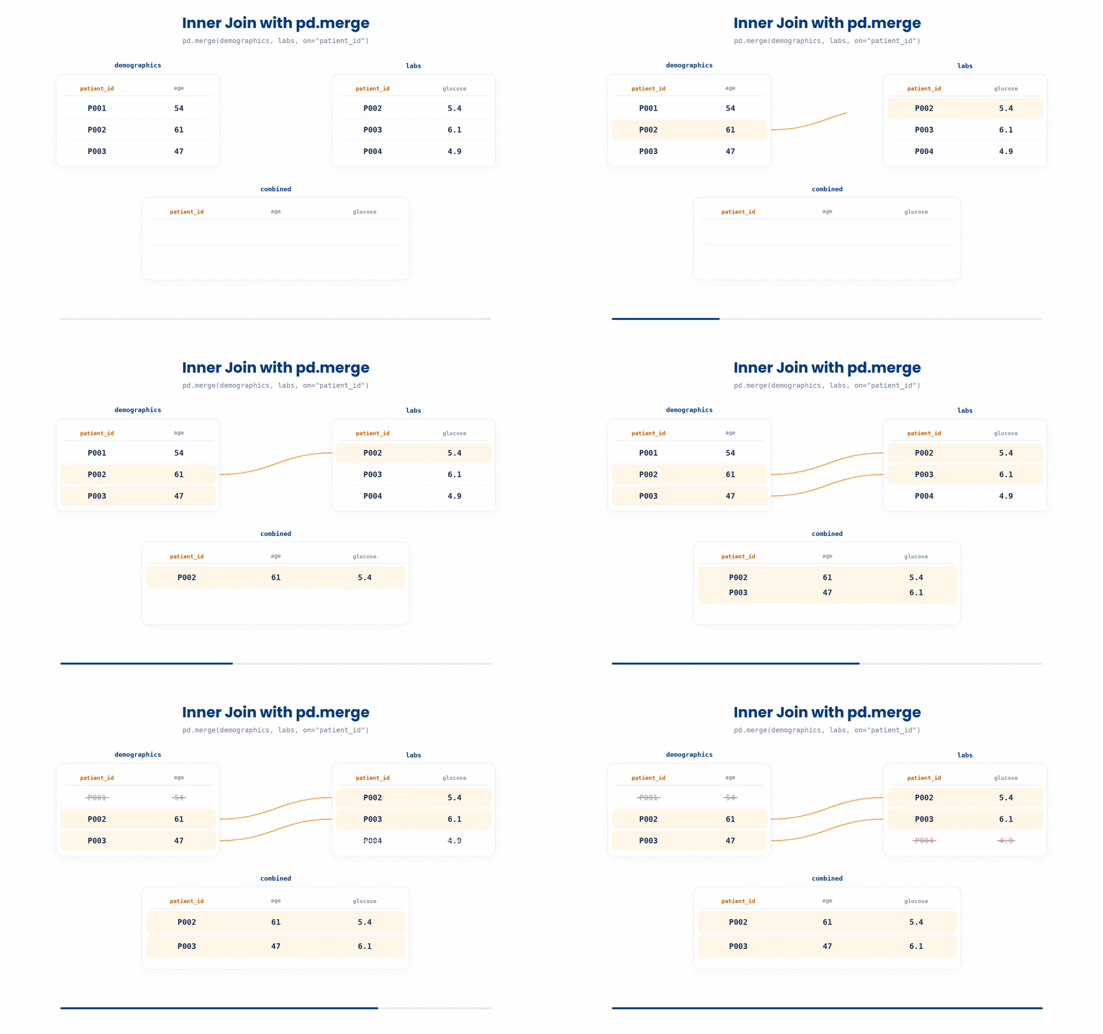
The default behaviour of pd.merge keeps only the rows that have a match on both sides. This is called an inner join, and it is what you want when only patients with both kinds of information matter for your analysis.
Try this snippet in the Python Scratchpad on the right.
import pandas as pd

demographics = pd.DataFrame({
 "patient_id": ["P001", "P002", "P003"],
 "age": [54, 61, 47],
})
labs = pd.DataFrame({
 "patient_id": ["P002", "P003", "P004"],
 "glucose": [5.4, 6.1, 4.9],
})
combined = pd.merge(demographics, labs, on="patient_id")
print(combined)Two patients survive the merge: P002 and P003, the two who appear in both tables. P001 (no labs) and P004 (no demographics) are dropped. That is the inner join's promise: every output row has a value in every column.
5.2 Left and outer join
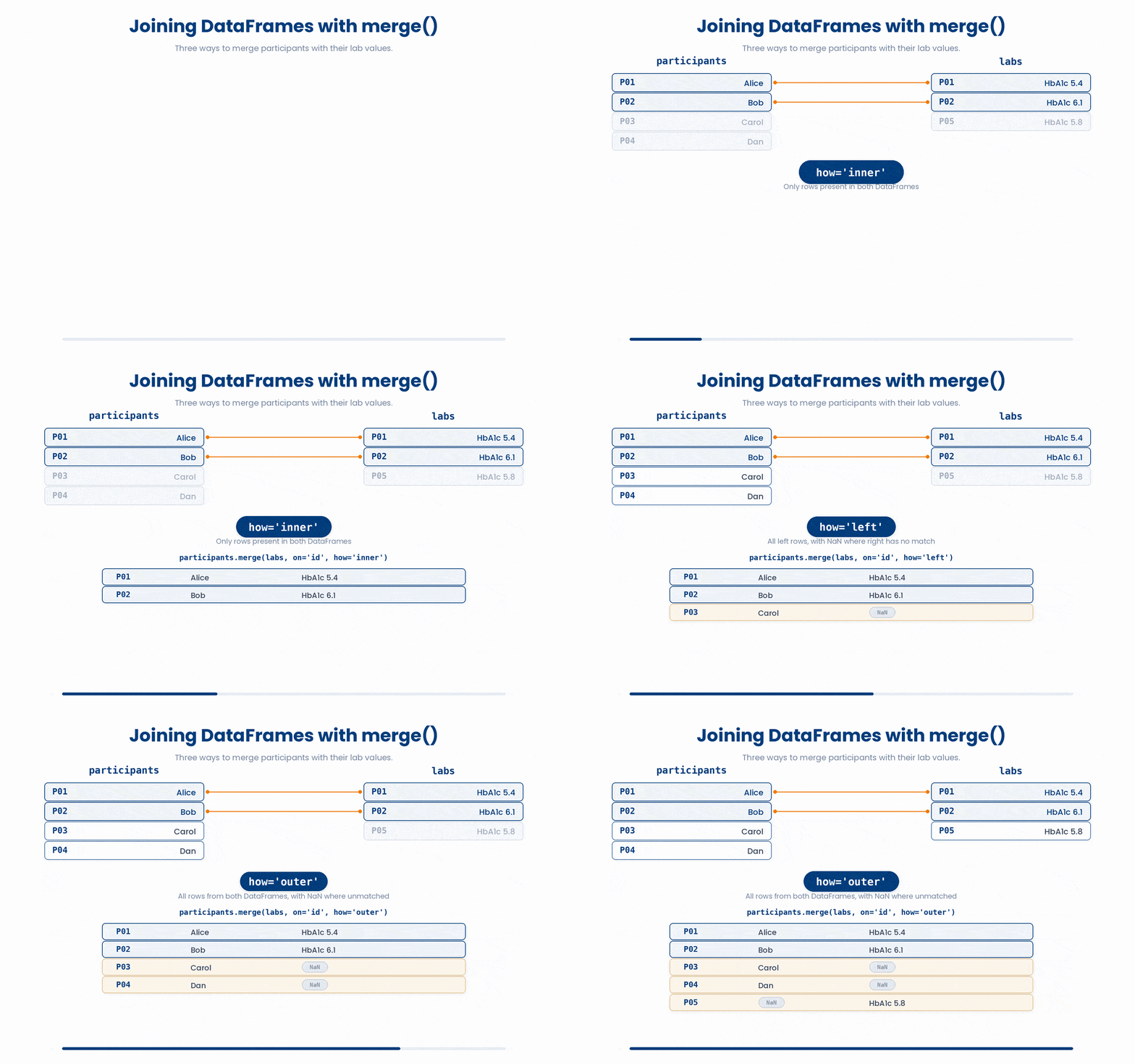
When that is too strict, you reach for one of the other join types. Pass how="left" to keep every row from the left table, filling NaN where the right table has no match. Pass how="right" for the mirror image. Pass how="outer" to keep every row from both (the union), with NaN wherever a side is missing.
Try this snippet in the Python Scratchpad on the right.
import pandas as pd

demographics = pd.DataFrame({
 "patient_id": ["P001", "P002", "P003"],
 "age": [54, 61, 47],
})
labs = pd.DataFrame({
 "patient_id": ["P002", "P003", "P004"],
 "glucose": [5.4, 6.1, 4.9],
})
left = pd.merge(demographics, labs, on="patient_id", how="left")
outer = pd.merge(demographics, labs, on="patient_id", how="outer")
print(left)
print(outer)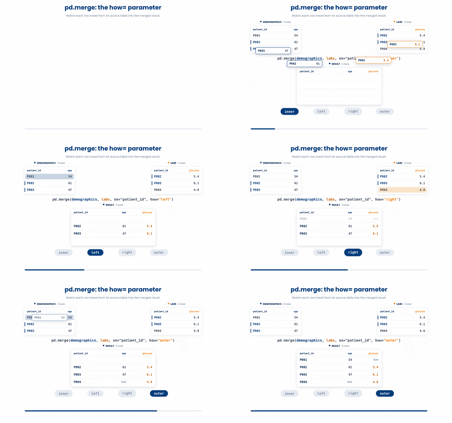
5.3 How to pick
How to pick. Inner is the right default when you want only complete records. Left is the right choice when one of the two tables is your primary list and you want to enrich it without losing anyone (a list of trial participants, say, getting annotated with whatever lab values exist for them). Outer is the right move when you are auditing two sources for completeness and need to see exactly which side each record came from.
If the key column has different names on each side, replace on= with the pair left_on= and right_on=. The shape is the same; pandas just stops assuming the names match.
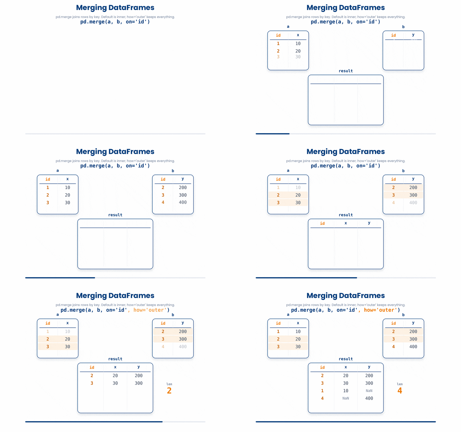
One trap to know about. If your key is not unique on one side (a patient with three lab visits, all under the same patient_id), every match on the unique side gets duplicated to line up with every match on the duplicated side. You can join a 100-row demographics table to a 300-row lab table and end up with 300 output rows: one per lab visit, each carrying its patient's demographics. That may be exactly what you want, or may be a shock. Check df["patient_id"].is_unique on each side before the merge and you will not be surprised.
6 One-hot encoding with pd.get_dummies
Many tools that accept a numeric feature matrix cannot consume a column of category labels directly. pd.get_dummies converts each categorical column into a set of 0/1 columns - one per category. Pass drop_first=True to drop one column per group, which is the convention when the columns will go into a regression with an intercept.
Try this snippet in the Python Scratchpad on the right.
import pandas as pd

df = pd.DataFrame({
    "patient_id": ["P001", "P002", "P003", "P004"],
    "clinic": ["A", "B", "A", "C"],
    "age": [54, 61, 47, 72],
})
print(pd.get_dummies(df, columns=["clinic"]))
print(pd.get_dummies(df, columns=["clinic"], drop_first=True))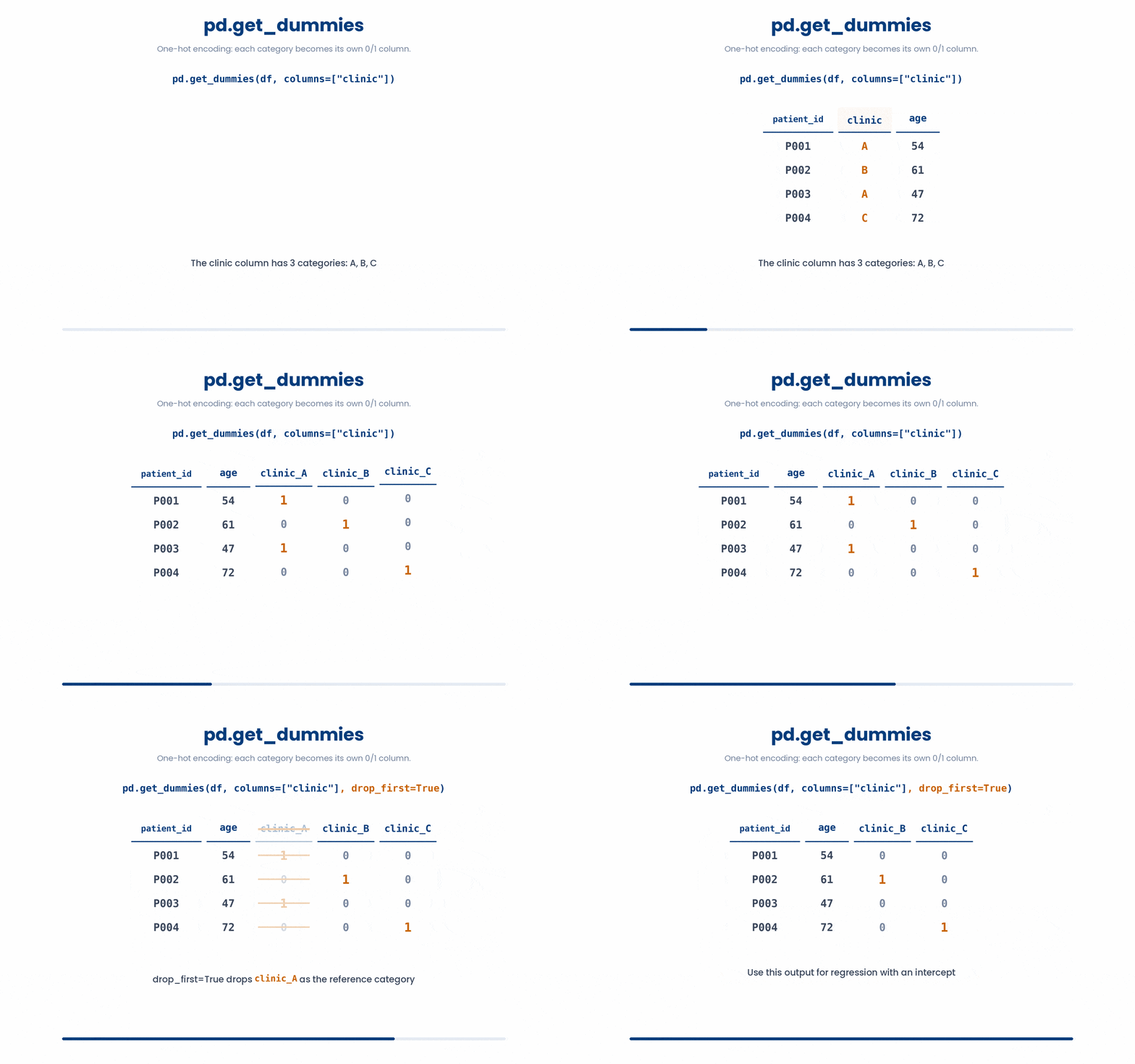
7 Building processing pipelines with method chaining
Most real analyses are not one pandas call but several in a row. Read the file, drop the missing rows, filter to a cohort, group by clinic, summarise, sort the result. You can write each step as its own line and store the intermediate DataFrames in named variables — and sometimes that is the right thing to do — but pandas methods almost all return a DataFrame, which means each method's output is another DataFrame ready to feed into the next method. Stringing the calls together is called method chaining, and the result is a single expression that reads top to bottom like a recipe.
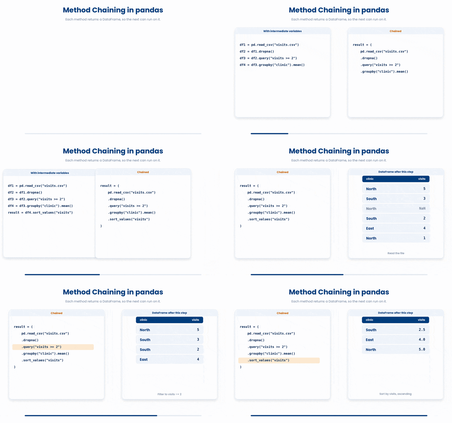
Here is the same analysis written first as a sequence of separate steps, then as a chain. The two produce the same result.
Try this snippet in the Python Scratchpad on the right.
import pandas as pd

df = pd.DataFrame({
    "clinic": ["A", "A", "B", "B", "B"],
    "age": [54, 47, 61, 72, 38],
    "bmi": [27.3, 31.2, 24.1, 22.8, 29.5],
})

# Unchained
filtered = df[df["age"] > 40]
grouped = filtered.groupby("clinic")["bmi"].mean()
result = grouped.sort_values(ascending=False)
print(result)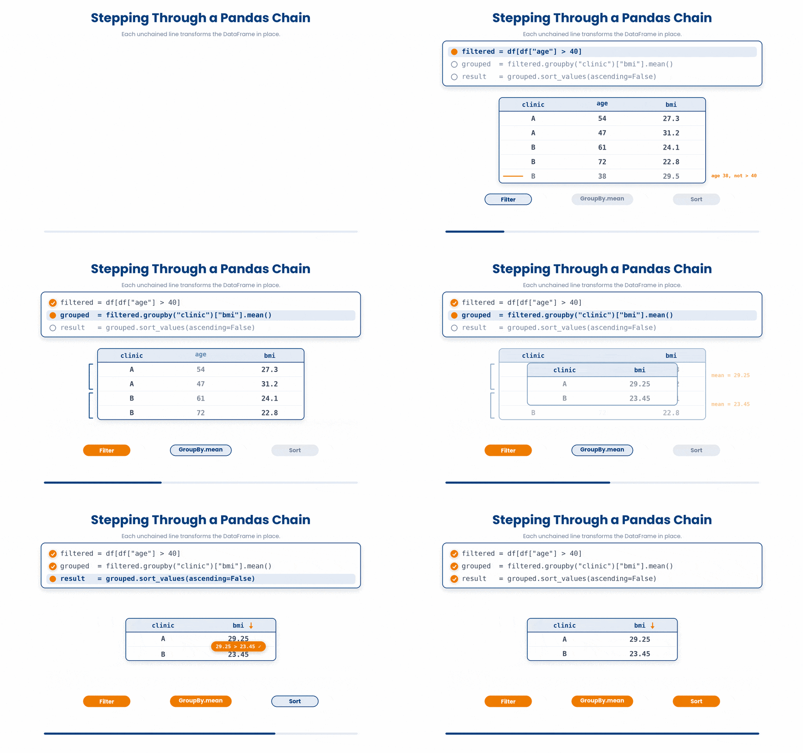
Try this snippet in the Python Scratchpad on the right.
import pandas as pd

df = pd.DataFrame({
    "clinic": ["A", "A", "B", "B", "B"],
    "age": [54, 47, 61, 72, 38],
    "bmi": [27.3, 31.2, 24.1, 22.8, 29.5],
})

# Chained
result = (
    df
    .loc[df["age"] > 40]
    .groupby("clinic")["bmi"]
    .mean()
    .sort_values(ascending=False)
)
print(result)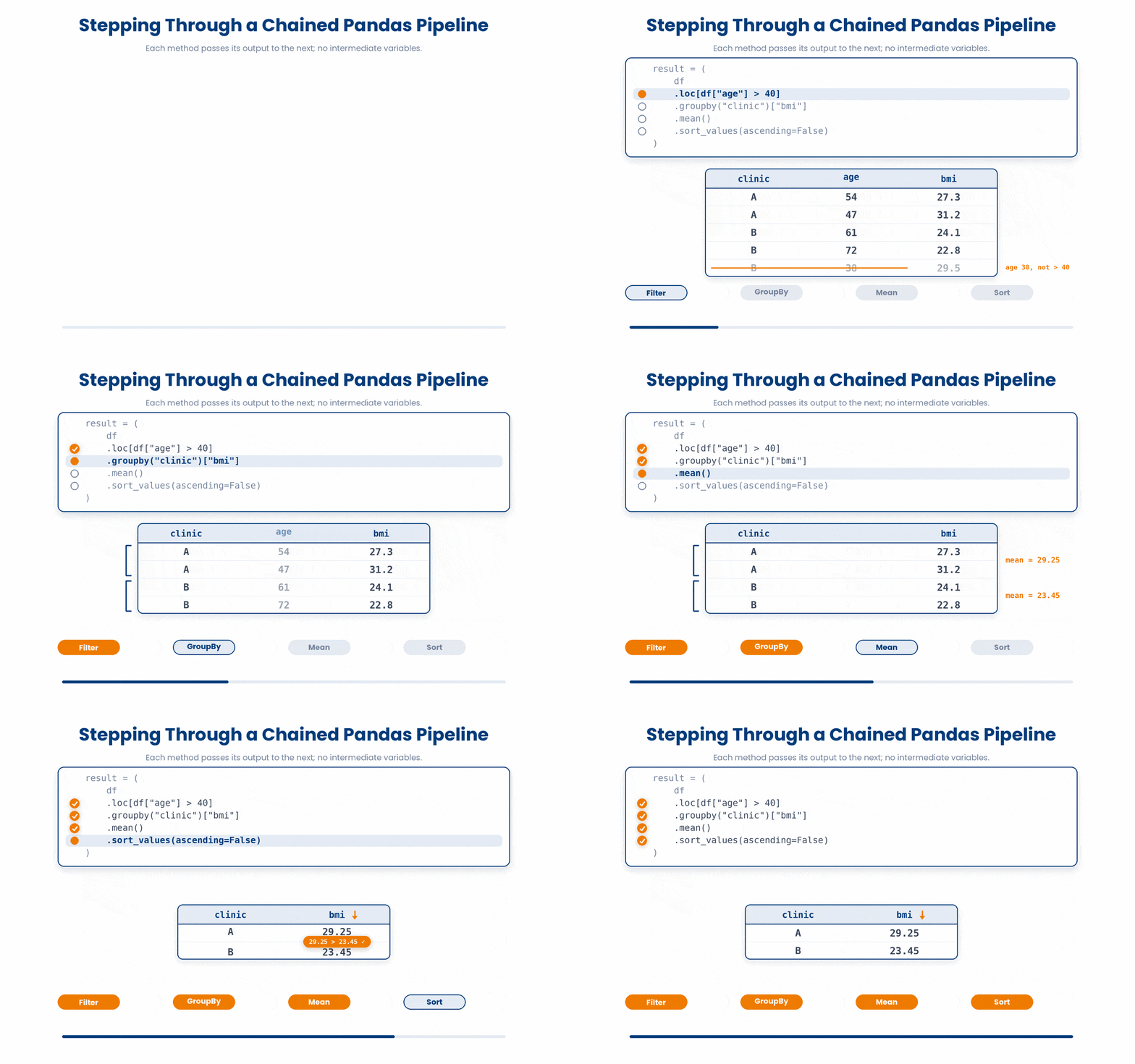
Method chaining is a fantastic way to express a flow of operations, but without strict formatting, a long chain quickly becomes unreadable.
Three rules make this layout highly readable:
- Wrap it in parentheses (): This allows Python to safely ignore the line breaks inside. Without them, you would need an ugly backslash (\) at the end of every line.
- Line up the dots vertically: This naturally guides the reader's eye downward through the sequence of operations.
- One method per line: This makes it incredibly easy to comment out a single step for debugging, or to insert a new step, without touching the rest of the code.
Because a method chain is a single continuous expression, you can't use standard assignment (like df['new_col'] = 5) in the middle of it.
To add a new column without breaking your chain, use .assign(). It evaluates your data and returns a brand-new DataFrame with the added column, allowing it to slot cleanly right into your pipeline.
Here it is running. Inside .assign(), each keyword argument names the new column, and its value is usually a lambda that takes the DataFrame at that point in the chain and returns the column to add.
Try this snippet in the Python Scratchpad on the right.
import pandas as pd

df = pd.DataFrame({
    "patient_id": ["P001", "P002", "P003"],
    "weight_kg": [72, 80, 65],
    "height_m": [1.75, 1.80, 1.60],
})
result = (
    df
    .assign(bmi=lambda d: d["weight_kg"] / d["height_m"] ** 2)
)
print(result)Write the lambda as lambda d: ..., taking the DataFrame as its argument, rather than reaching for the original df by name inside .assign(). The reason is what d actually is: the DataFrame as it stands at that exact point in the chain, after any .dropna() or filter earlier in the same chain has already run. Refer to the original df by name instead and you silently reach back past that filter — the calculation runs on rows the chain was supposed to have removed.
Try this snippet in the Python Scratchpad on the right.
import pandas as pd

df = pd.DataFrame({
    "patient_id": ["P001", "P002", "P003", "P004"],
    "clinic": ["A", "A", "B", "B"],
    "weight_kg": [72, 58, 65, 90],
})

# Safe: the lambda sees the DataFrame as it stands after the filter, so
# .sum() only adds up clinic A's own two weights.
safe = (
    df
    .loc[df["clinic"] == "A"]
    .assign(pct_of_group=lambda d: d["weight_kg"] / d["weight_kg"].sum() * 100)
)
print(safe)

# Risky: df here still names the ORIGINAL four-row table, so .sum() silently
# adds up all four patients, not just the filtered two.
risky = (
    df
    .loc[df["clinic"] == "A"]
    .assign(pct_of_group=df["weight_kg"] / df["weight_kg"].sum() * 100)
)
print(risky)The three combine naturally in one pipeline. .dropna() clears the rows that are missing something the rest of the chain needs, .rename(columns=...) relabels a column so the result reads cleanly, and .assign() derives the column you actually want — in that order, because cleaning first means the rename and the derived column never have to deal with the rows you are about to throw away.
Try this snippet in the Python Scratchpad on the right.
import pandas as pd

df = pd.DataFrame({
    "patient_id": ["P001", "P002", "P003", None],
    "weight_kg": [72, 80, 65, 90],
    "height_m": [1.75, 1.80, None, 1.95],
})

clean = (
    df
    .dropna(subset=["patient_id", "height_m"])
    .rename(columns={"patient_id": "id"})
    .assign(bmi=lambda d: d["weight_kg"] / d["height_m"] ** 2)
)
print(clean)Something important to note. Method chaining is a tool for readability. If your pipeline grows past five or six steps, or if you need to inspect an intermediate result to see what is going wrong, it is time to break the chain. Saving your progress back into named variables is often the clearer choice.
8 From pandas to NumPy and back
Once your data is clean inside a DataFrame, the bridge into the NumPy world is .to_numpy() (or its older alias .values). It returns the underlying 2D array with the index and column labels dropped. Going the other way, pd.DataFrame(arr, columns=[...]) wraps an array back into a DataFrame with named columns.
Try this snippet in the Python Scratchpad on the right.
import pandas as pd
import numpy as np

df = pd.DataFrame({"age": [54, 61, 47], "bmi": [27.4, 31.1, 24.8]})
arr = df.to_numpy()
print(arr)
print(arr.shape)

back = pd.DataFrame(arr, columns=["age", "bmi"])
print(back)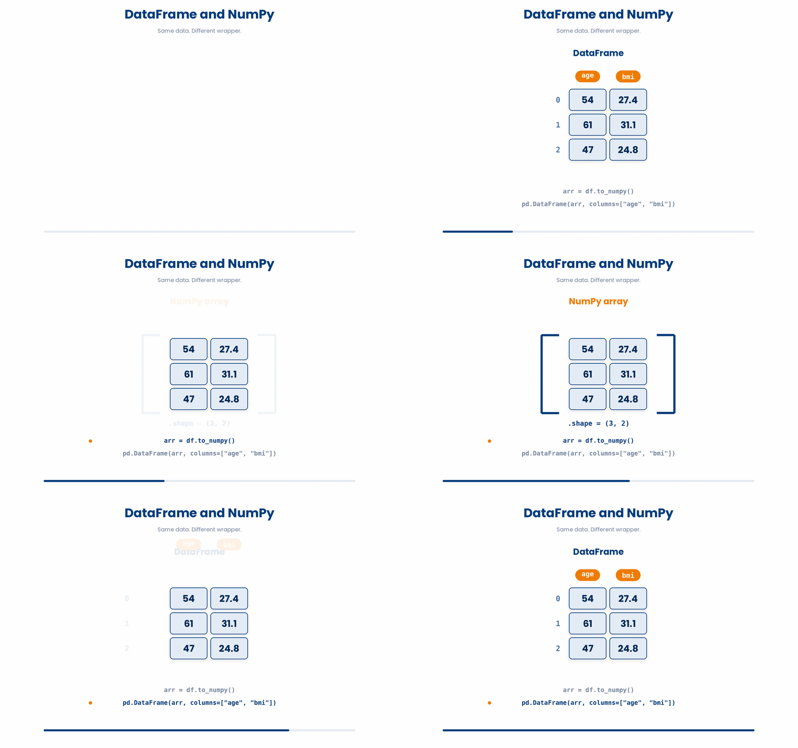
The bridge runs the other way too, and most of the time you do not need to cross it on purpose. A pandas Series stores its values in a NumPy array underneath, so a NumPy function handed a Series reads that array directly and hands back a Series, index and all — no .to_numpy() needed first. np.log(df["glucose"]) is a Series, not a plain array.
Try this snippet in the Python Scratchpad on the right.
import pandas as pd
import numpy as np

df = pd.DataFrame({
    "patient_id": ["P001", "P002", "P003"],
    "glucose": [5.4, 6.1, 4.9],
})
df["log_glucose"] = np.log(df["glucose"])
print(df)
print(type(np.log(df["glucose"])))Every rule from the NumPy module carries over unchanged. Element-wise arithmetic on a column works exactly like it does on an array — one calculation per row, no loop. A comparison like df["glucose"] > 7 returns a boolean Series the same way a comparison on an array returns a boolean array. And np.where reads a column just as happily as it reads an array.
Try this snippet in the Python Scratchpad on the right.
import pandas as pd
import numpy as np

df = pd.DataFrame({
    "patient_id": ["P001", "P002", "P003", "P004"],
    "glucose": [5.4, 7.8, 6.1, 9.2],
})
df["glucose_mgdl"] = df["glucose"] * 18
print(df["glucose"] > 7)
df["flag"] = np.where(df["glucose"] > 7, "high", "normal")
print(df)9 Putting it together
The six tools in this part are the workflow you reach for at the end of an analysis — once your data is clean, you reshape it, combine it with what else you have, encode the categorical pieces, chain everything into one expression, and hand it off to the next stage as a NumPy array.
Work through this example in three stages. You unlock each stage only after the tutor confirms the previous one. Each stage removes more of the scaffolding — by the end you are writing it yourself.
Problem: You have patients.csv (one row per patient, with clinic and demographics) and labs.csv (multiple rows per patient, one per lab visit). Read both, summarise labs per patient (mean glucose), left-merge the summary back onto patients, one-hot encode the clinic column, and convert the resulting feature DataFrame into a NumPy array ready for the next tool.
import pandas as pd

patients = pd.read_csv("patients.csv")
labs = pd.read_csv("labs.csv")
lab_summary = labs.groupby("patient_id", as_index=False)["glucose"].mean()

X = (
    patients
    .merge(lab_summary, on="patient_id", how="left")
    .pipe(pd.get_dummies, columns=["clinic"], drop_first=True)
    .drop(columns=["patient_id"])
    .to_numpy()
)
print(X.shape)- First we load both tables and collapse the long labs table to one row per patient by grouping on patient_id and taking the mean glucose.
- Then we build the feature matrix as one chained pipeline: a left merge keeps every patient (even those with no labs), and .pipe(pd.get_dummies, ...) one-hot encodes the clinic column with drop_first=True to avoid the dummy-variable trap.
- Finally we drop patient_id (an identifier, not a feature) and call .to_numpy() to hand the matrix off to the next tool. Printing .shape confirms the number of rows and feature columns.
The same solution with key parts replaced by ???.
Fill in every ??? so the code matches the reference,
then ask the tutor to check it.
Your turn: You now have students.csv (200 rows, columns: student_id, age, school, gpa — 4 unique schools) and grades.csv (multiple rows per student, columns: student_id, score). Aggregate grades to one mean score per student, left-merge onto students, one-hot encode school with drop_first=True, drop student_id, convert to a NumPy array, and print its shape.
10 Check your understanding
You have reached the end of the module. Try the same questions again — your answers here, paired with your pre-test answers, are how we measure what the module taught you. Answer every question and confidence rating, then click Submit and see results to view your score.
You have a wide DataFrame with columns patient_id, v1, v2, v3 (weights at three visits). Which call turns it into long form with one row per (patient, visit, weight)?
You have a long DataFrame with columns patient_id, timepoint, weight. Which call turns it into wide form — one row per patient, one column per timepoint?
pd.crosstab(df["clinic"], df["sex"]) returns what?
You merge a one-row-per-patient demographics table with a multiple-rows-per-patient labs table using an inner join on patient_id. How many rows does the result have?
You want to keep EVERY row of the demographics table, attaching lab values where a patient has them and NaN where they do not. Which how= do you pass to pd.merge?
pd.get_dummies(df, columns=["clinic"]) does what to the DataFrame?
What is the role of the round brackets in a chained pandas pipeline like (df.pipe(...).merge(...).assign(...))?
df.to_numpy() on a DataFrame of numeric columns returns what?
I can pivot a long-form DataFrame to wide form and melt a wide-form DataFrame to long form.
I can merge two tables on a key column and pick the right join type (inner, left, full outer) for the question I am asking.
I can write a small chained pipeline that joins two tables, one-hot encodes the categorical columns, and bridges into NumPy with .to_numpy().
11 Your results
Here is how your post-test answers compare with your pre-test answers. The pre/post pairing is the most reliable way to see what this module actually taught you.
Submit the post-test to see your results.
What is the one thing from this module that is still unclear to you?