

1 Before you start
This is not graded, and it does not count towards anything. Answer every question even if you are only guessing — having a go at something before you have been taught it is one of the best ways to remember it afterwards. The lesson ends with another short check, and there you will be shown the correct answer for anything you missed. Choose an option for every question and confidence rating, then click Submit answers.
You write df = pd.DataFrame({"a": [1, 2, 3], "b": [10, 20, 30]}). What does df["a"] return?
Which of these reads a tab-separated file into a DataFrame?
A column of strings like "2024-01-15" is in your DataFrame. After running df["d"] = pd.to_datetime(df["d"]), what dtype does d have?
Which call reports the dtype and the number of non-null values for every column of df?
df["clinic"].value_counts() returns which kind of object?
A DataFrame is indexed by patient_id ("P001", "P002", "P003", ...). Which call returns the row for patient "P002"?
You want every row in df where age > 50 AND bmi > 25. Which expression is correct?
You want every row whose clinic is one of "A", "B", or "C". Which expression works?
I can read a CSV or Excel file into a DataFrame and use head, info, and describe to get a quick feel for what is in it.
I can filter a DataFrame on one or more boolean conditions and pull out the rows that match.
I can parse a column of date strings with pd.to_datetime and pull out the year or month with .dt.
2 Introduction
Pandas is the workhorse of data analysis in Python. Almost any tabular data you will meet in precision medicine — patient records, lab results, gene counts, survey responses — lives most comfortably in a pandas DataFrame.
This is the first of three parts on pandas. Part I focuses on getting data into a DataFrame and understanding it. Part II covers cleaning and transforming a single DataFrame. Part III covers reshaping, combining, and exporting.
This part covers seven connected pieces. Treat them as a path — each one builds on the one before, and by the end you can read a real CSV, look it over, and pull out the rows that matter for the question you are asking.
- Introduction to Pandas DataFrames — what a DataFrame is, how to build one from scratch, and what a Series is.
- Reading CSV and Excel files — pull a real file off disk in one line.
- Working with dates:
pd.to_datetime— parse a column of date strings into proper datetime values you can sort and filter on. - Inspecting dataframes — the four short calls (
head,shape,info,describe) that tell you what you have. - Counting categories with
value_counts— the call you reach for most often on a categorical column. - Data selection and filtering — pick the rows and columns you actually want, by label, by position, or by condition.
- Filtering by multiple categories with
.isin— keep every row whose value matches one of a list, in one short expression.
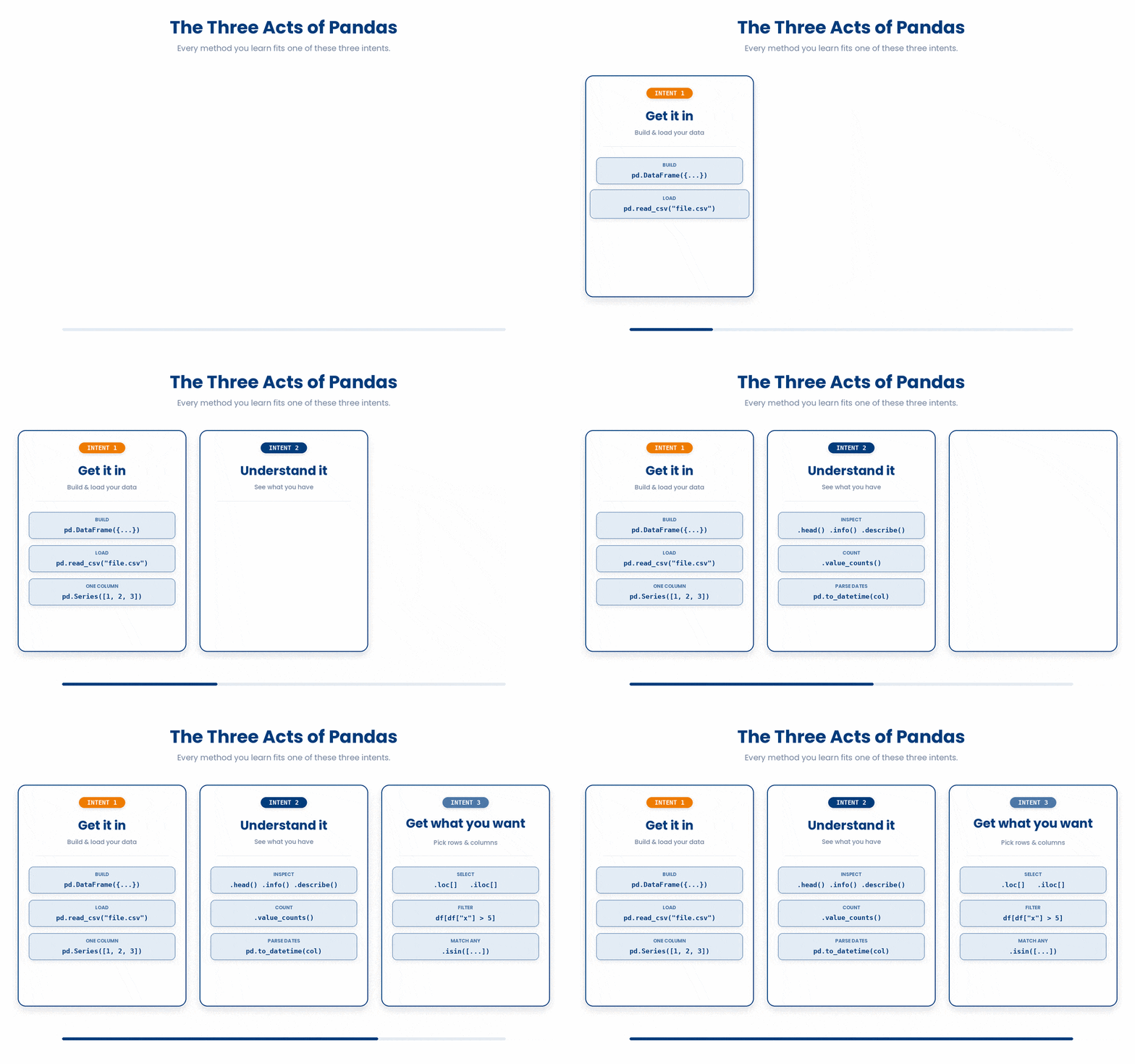
Try every snippet in the Python Scratchpad on the right. By the end of this part you will read a CSV, inspect it, parse its dates, and pull out the rows that matter.
3 Introduction to Pandas DataFrames
A DataFrame is the central object in pandas. Picture it as a table with named columns, numbered rows, and a value in every cell.
By convention, pandas is imported under the short alias pd, so the line at the top of your script will look the same as the line at the top of everyone else's:
Try this snippet in the Python Scratchpad on the right.
import pandas as pd

data = {
    "patient_id": ["P001", "P002", "P003"],
    "age": [54, 61, 47],
    "bmi": [27.3, 24.1, 31.2],
}
df = pd.DataFrame(data)
print(df)Each entry in data becomes a column: the name on the left is the column header, and the list on the right fills the cells beneath it.
The 0, 1, 2 down the left side is the index, which pandas adds for you when you do not specify one. Naming the variable df is another convention you will see everywhere.

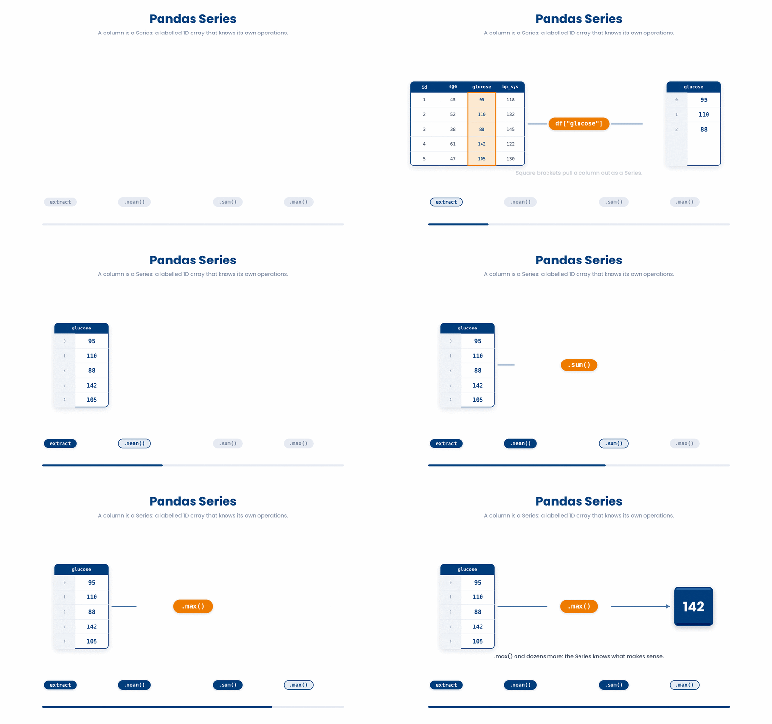
A single column is its own object, called a Series: a one-dimensional labelled array, or a list of values with an index attached. You pull one out of a DataFrame by passing the column name in square brackets.
That last line shows why pandas is worth the import. Once your data is in a Series, calling .mean() gives you the average. No loop, no sum divided by length, no manual conversion to floats. The Series knows its own values and the operations that make sense on them. The same applies to .sum(), .median(), .std(), .min(), .max(), and dozens of others.
Building a DataFrame from a dictionary is fine for examples and tiny tables, but real data almost always lives in a file. The next subtopic covers how to load one.
4 Reading CSV and Excel files with Pandas
Almost no real-world data starts its life as a Python literal. Instead, it arrives as a CSV from a colleague, an Excel workbook from a clinical study, or a TSV exported from a genomic sequencing pipeline. Fortunately, pandas can read all of these formats with a single, easily memorable line of code.
To load a comma-separated file, use the pd.read_csv() function. Simply pass in the file path, and pandas handles the heavy lifting: it identifies the columns from the header row, infers the data type for each column, and returns a fully structured DataFrame.
Note: We have provided several csv files that have beep pre-loaded for you in the Python Scratchpad
Try this snippet in the Python Scratchpad on the right.
import pandas as pd

df = pd.read_csv("patients.csv")
print(df)Several keyword arguments to read_csv come up so often that they are worth knowing on day one:
sep="\t"reads a tab-separated file (TSV) instead of the default comma.header=Nonetellspandasthe file has no header row, so it should make up column names itself.index_col="patient_id"uses a specific column as the row index instead of the auto-numbered0,1,2.na_values=["NA", "missing", -999]tellspandaswhich strings to treat as missing (more on missing values in a later subtopic).nrows=100reads only the first hundred rows, perfect for a quick peek at a huge file before you commit to loading the whole thing.
Try this snippet in the Python Scratchpad on the right.
import pandas as pd

df = pd.read_csv(
    "patients.tsv",
    sep="\t",
    index_col="patient_id",
    na_values=["NA", "missing", -999],
    nrows=100,
)

print(df)Excel files use a sister function called. pd.read_excel. The shape is the same. Excel workbooks can have multiple sheets, so the extra argument you reach for most often is sheet_name: pass the sheet's name as a string, or its position as an integer (0 for the first sheet).
Writing a DataFrame back out is the mirror image.
df.to_csv("output.csv")writes a CSVdf.to_excel("output.xlsx")writes an Excel file.
One small habit worth forming: pass index=False unless the index carries information. Without it, pandas writes the row numbers as a first column, which the next person to read your file will then have to clean up.
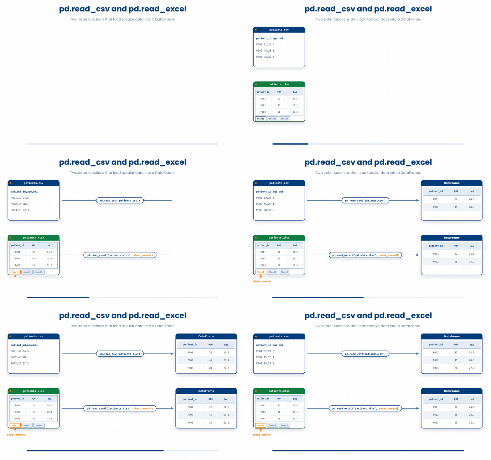
The syntax to import Excel or CSV files as Dataframes is given as below.
df.to_csv("output.csv", index=False)
df.to_excel("output.xlsx", index=False)
If you get a FileNotFoundError, pandas is looking in your current working directory. Either move the file there, pass a full path, or use pathlib to build a path from the script's location. The easiest first move is print(__file__) at the top of your script to remind yourself where Python thinks it is running from.
Real data is often published at a web address rather than sitting on your own disk — a public health dataset, a government release, a colleague's shared file. Outside this Scratchpad, reading one is nothing new: pd.read_csv(url), with the URL standing in for a file path.
Inside this Scratchpad, that line alone fails. The Scratchpad runs Python inside your browser, and a browser will not let a page reach out to the network on its own — that restriction belongs to the browser sandbox this code runs in, not to pandas. The fix is one extra import: from pyodide.http import open_url, then wrap the URL in open_url(...) before handing it to read_csv.
Try this snippet in the Python Scratchpad on the right.
from pyodide.http import open_url
import pandas as pd

url = "https://raw.githubusercontent.com/mwaskom/seaborn-data/master/iris.csv"
df = pd.read_csv(open_url(url))
print(df.shape)
print(df.head())Everywhere else in this course, pd.read_csv("patients.csv") is enough, because those files are already preloaded for you. Reach for open_url only when the data genuinely lives outside the Scratchpad, at a real web address.
5 Working with dates: pd.to_datetime
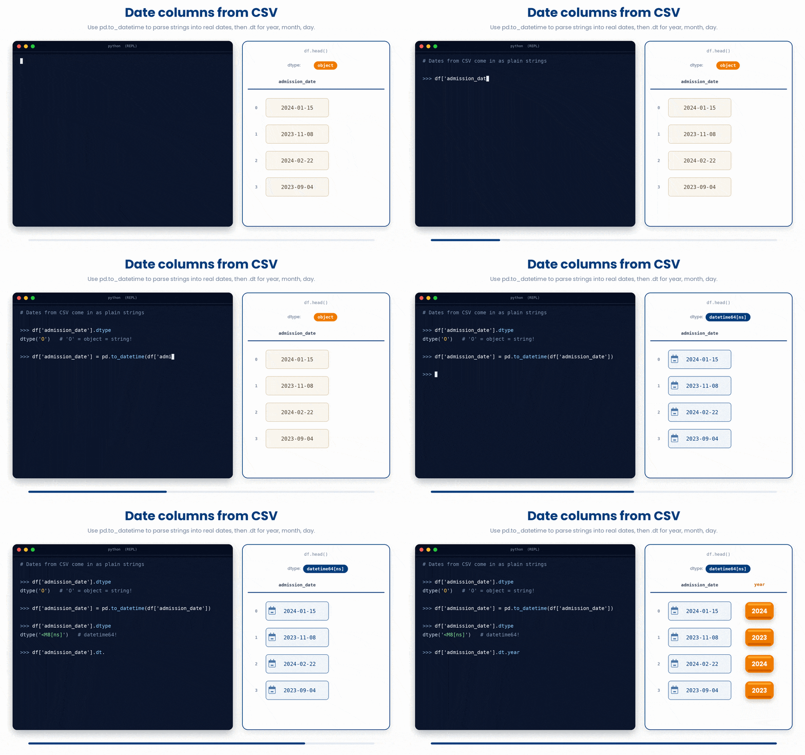
A column of dates that comes out of CSV is almost always a string. pandas does not know that "2024-01-15" is a date until you tell it.
The pd.to_datetime function parses a column into proper datetime values. Once converted, you can easily sort by date, filter by specific ranges, and extract the year, month, or day using the .dt accessor. Proper date handling is essential in clinical data, where you constantly manage admission dates, follow-up intervals, and dates of birth.
Try this snippet in the Python Scratchpad on the right.
import pandas as pd

df = pd.DataFrame({
    "patient_id": ["P001", "P002", "P003"],
    "visit": ["2024-01-15", "2024-03-02", "2024-06-21"],
})
df["visit"] = pd.to_datetime(df["visit"])
print(df.dtypes)
print(df["visit"].dt.year)
print(df["visit"].dt.month_name())pd.to_datetime becomes trustworthy once you add two keyword arguments that most first attempts leave out.
format="%d/%m/%Y"states the layout you expect. Without it,pandasguesses — and a date written03/04/2024is the 3rd of April to a British reader and the 4th of March to an American one. The guess happens silently, either way.errors="coerce"turns anything it cannot parse intoNaT, the datetime equivalent ofNaN, instead of raising an exception. One bad value out of ten thousand rows then costs you one missing entry, not a crashed script.
Try this snippet in the Python Scratchpad on the right.
import pandas as pd

df = pd.DataFrame({
    "patient_id": ["P001", "P002", "P003", "P004"],
    "visit": ["15/01/2024", "02/03/2024", "not a date", "21/06/2024"],
})
df["visit"] = pd.to_datetime(df["visit"], format="%d/%m/%Y", errors="coerce")
print(df)
print(df["visit"].isna().sum())Always check that count after converting a date column, with .isna().sum(). If the number of failures is larger than you expected, the usual cause is not messy data — it is the wrong format string for what the column actually contains.
6 Inspecting dataframes (head, info, describe)
The first thing you should do with any newly loaded DataFrame is inspect it.
Printing the entire dataset is counterproductive. This is because a DataFrame can hold millions of rows and will quickly clutter your screen with unreadable text.
Instead, use these method calls to immediately understand what you are working with. Run them in this order on every new file. If something is wrong, you will catch it early on, before the error propagates through the rest of your analysis.
df.head()shows the first five rows.df.head(10)shows the first ten.df.tail()shows the last five, useful for spotting a stray totals row at the bottom of a spreadsheet.df.shapeis a tuple of(rows, columns), no parentheses, it is an attribute, not a method.df.columnslists the column names.df.dtypesshows the type of each column.
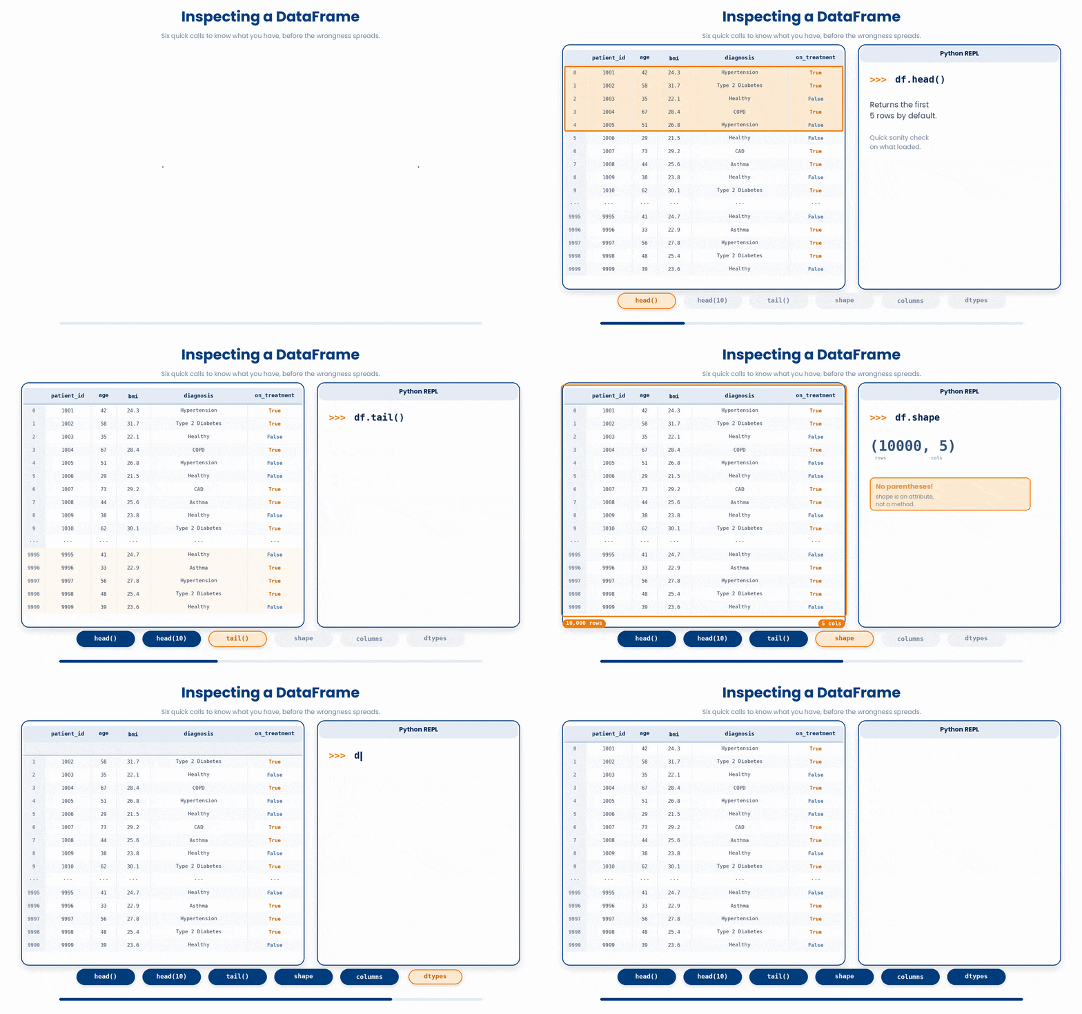
Try this snippet in the Python Scratchpad on the right.
import pandas as pd

df = pd.read_csv("patients.csv")
print(df.shape)
print(df.columns)
print(df.dtypes)
print(df.head())The df.info() method bundles these diagnostics together, adding the count of non-null values per column and the total memory usage of the DataFrame. It is the single most useful tool when an import goes wrong. For instance, if a column you expected to be numeric shows up as an object, df.info() flags it immediately.
Try this snippet in the Python Scratchpad on the right.
import pandas as pd

df = pd.read_csv("patients.csv")
df.info()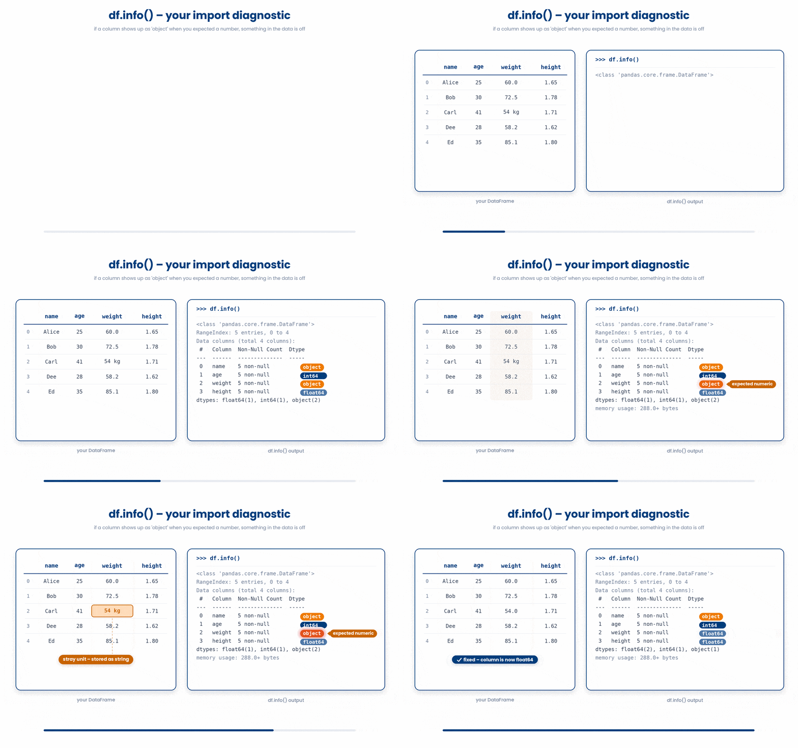
df.describe() gives you summary statistics for every numeric column at once: count, mean, standard deviation, minimum, the 25th, 50th, and 75th percentiles, and the maximum. It is the fastest way to spot impossible values — a negative age, a heart rate of zero, a BMI of 9000 — that always seem to lurk in real data.
For the non-numeric columns, df.describe(include="object") gives you count, number of unique values, the most frequent value, and how often it occurs.

Try this snippet in the Python Scratchpad on the right.
import pandas as pd

df = pd.DataFrame({
    "age": [54, 61, 47, 72, 38],
    "bmi": [27.3, 24.1, 31.2, 22.8, 29.5],
})
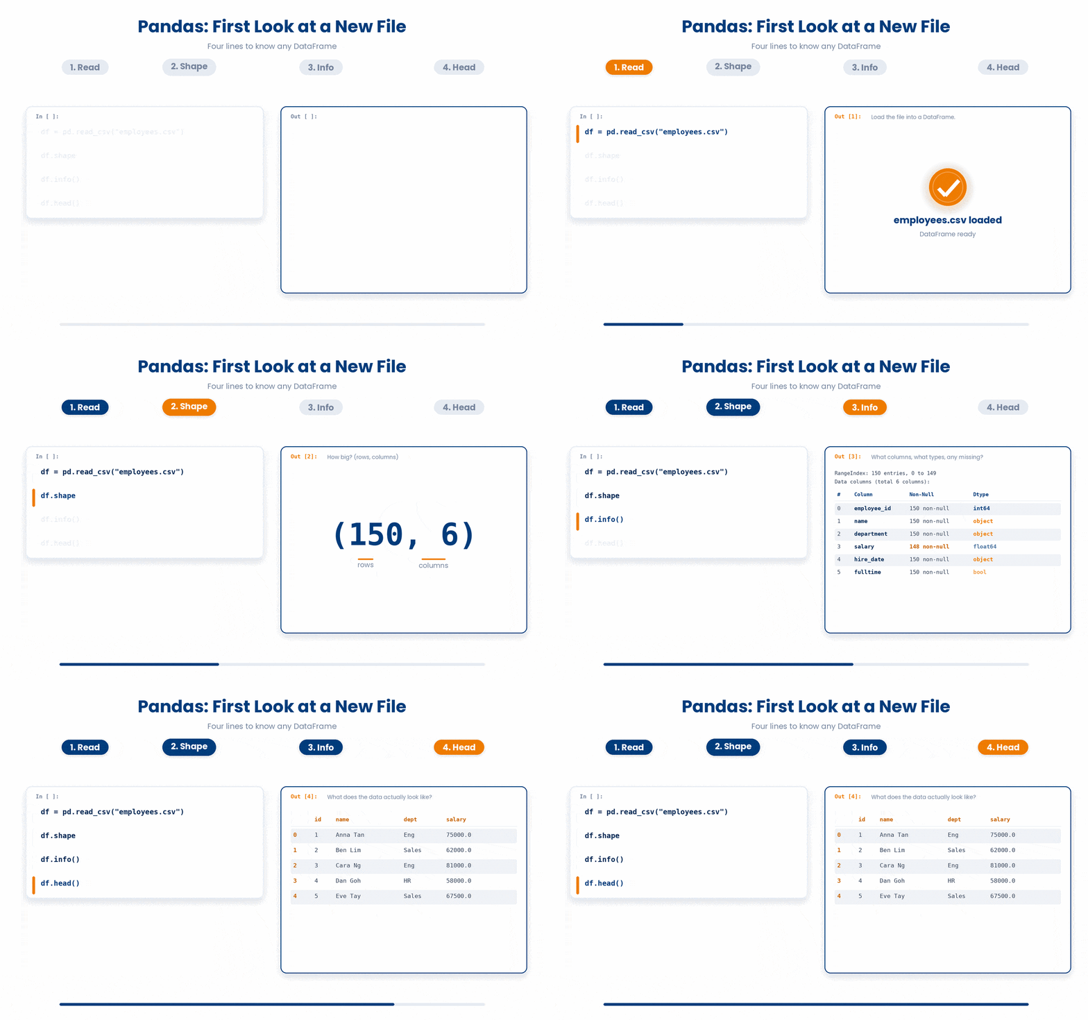
print(df.shape)A typical first pass on a new file is exactly four lines:
- read the file,
- print the shape,
- print info,
- print head.
Five seconds of looking saves an hour of debugging.
7 Counting categories with value_counts
When a column holds categorical values, smoking status, treatment arm, blood type, the question you ask first is almost always "what are the categories and how often does each one show up?"
Eyeballing head() will not tell you, because the first five rows might all happen to be the same category. You need a count over the whole column.
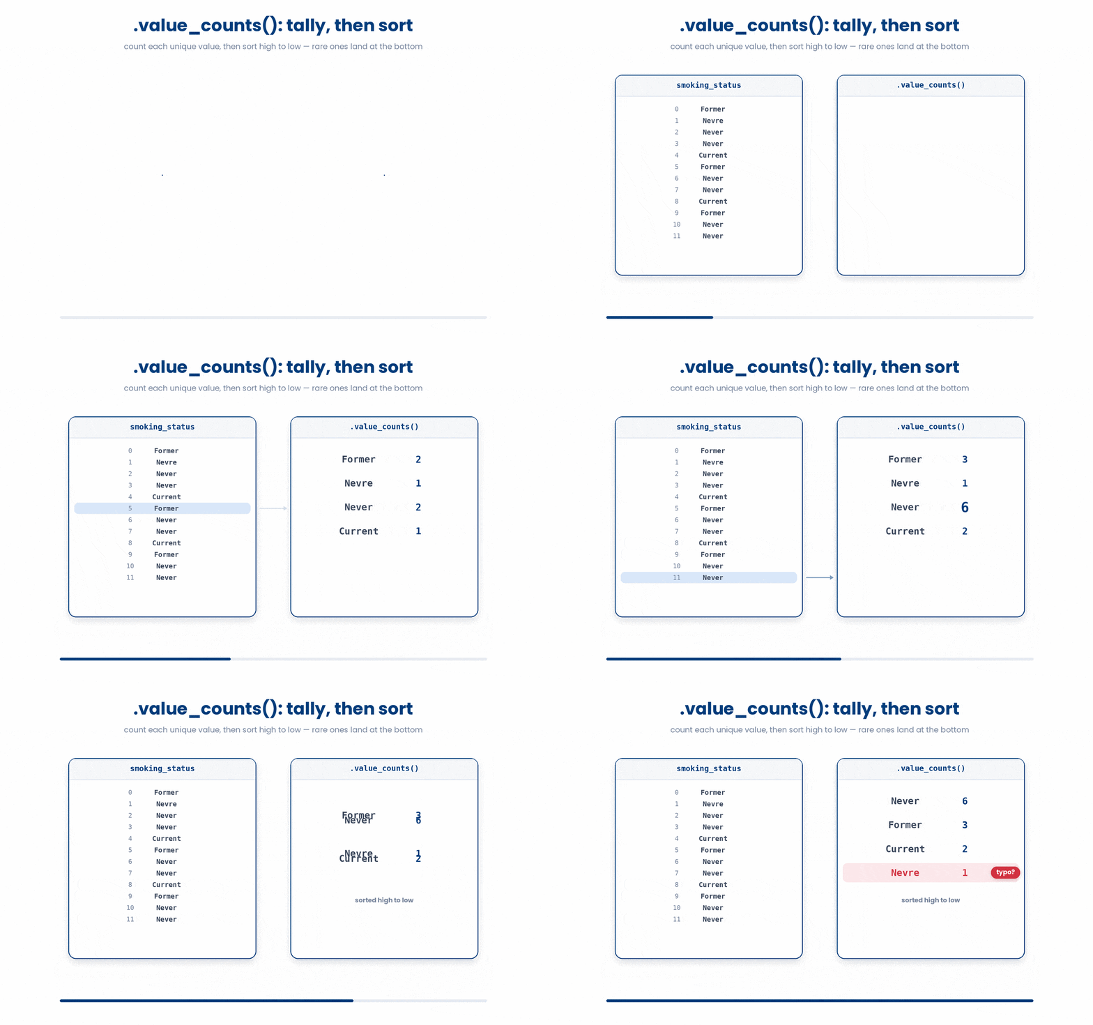
The call you reach for is .value_counts(). It returns a Series of counts, one per unique value, sorted high to low.
That ordering matters. The most common categories sit at the top where you will see them, and rare ones (often the interesting ones, or the data-entry typos) sit at the bottom where they stand out.
Two keyword arguments are worth knowing from the start.
normalize=Truereturns proportions instead of raw counts, useful when you want to compare the distribution across two cohorts of different sizes.dropna=Falsemakes missing values a category of their own and counts them alongside the rest, which is what you want when you are auditing data quality rather than describing the observed sample.
Try this snippet in the Python Scratchpad on the right.
import pandas as pd

df = pd.DataFrame({"clinic": ["A", "B", "A", "C", "B", "B", "A"]})
print(df["clinic"].value_counts())
print(df["clinic"].value_counts(normalize=True))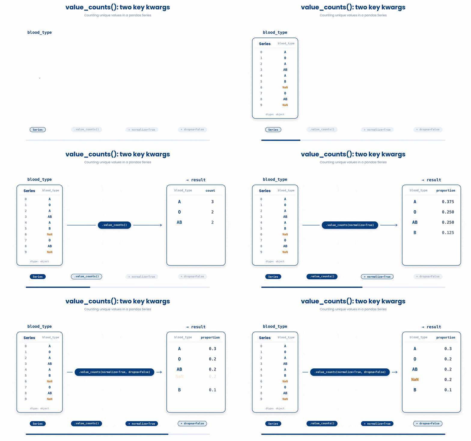
8 Data selection and filtering
You almost never want the entire DataFrame. You want the patients over sixty, the rows where BMI is above thirty, or the two columns called age and bmi but not the other twenty. pandas gives you a small set of notations for picking out the bits you care about, and they cover almost every selection you will ever make.
8.1 Picking columns
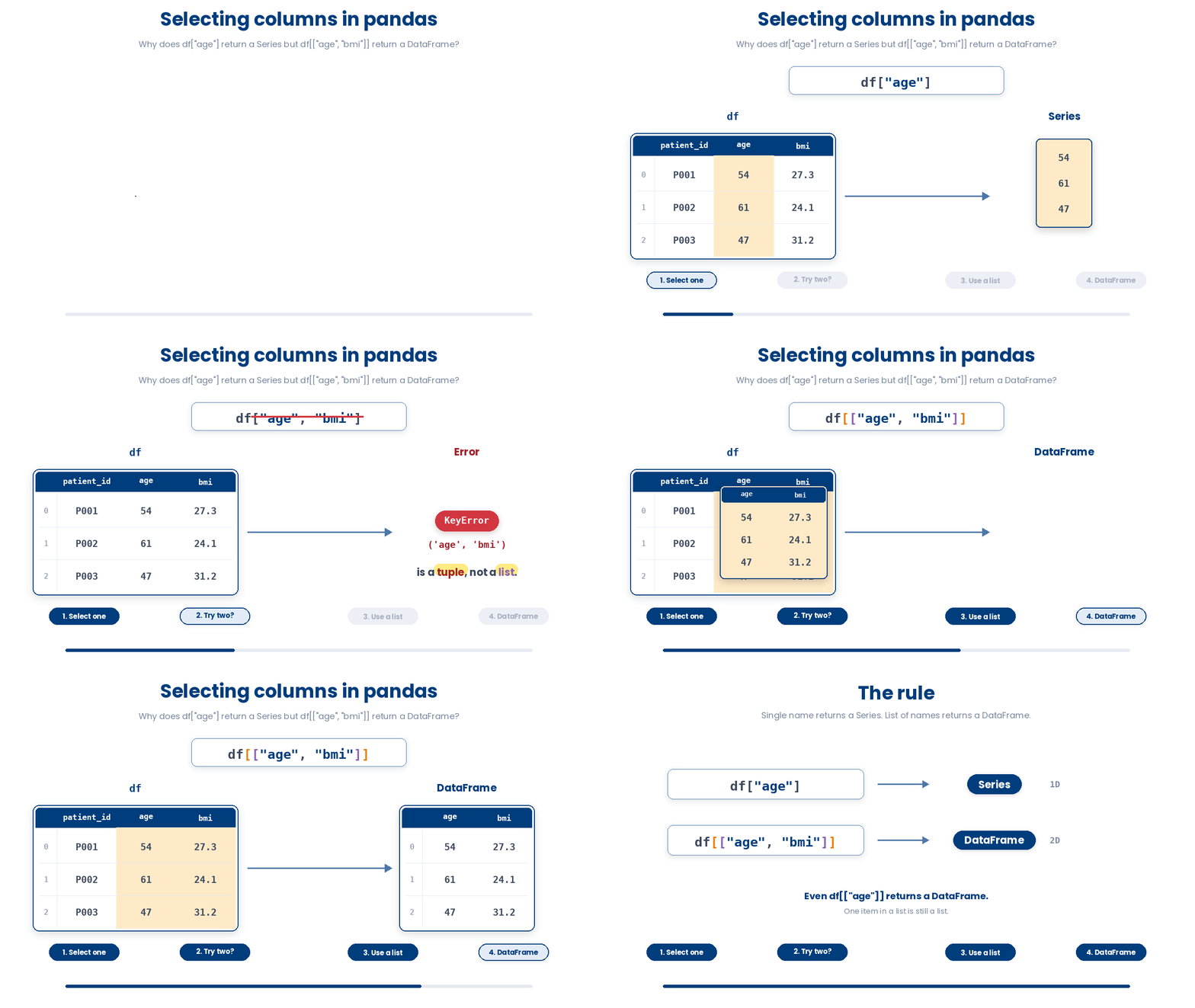
When selecting columns in pandas, the number of brackets you use determines what you get back. If you ask for a single column with df["age"], pandas hands you back a 1D Series. But if you want multiple columns, you must use double square brackets—like df[["age", "bmi"]]—which returns a smaller 2D DataFrame. If the double brackets look strange, just remember that the outer pair tells pandas you want to select data, while the inner pair is simply a standard Python list of the column names you are asking for.
Try this snippet in the Python Scratchpad on the right.
import pandas as pd

df = pd.DataFrame({
    "patient_id": ["P001", "P002", "P003"],
    "age": [54, 61, 47],
    "bmi": [27.3, 24.1, 31.2],
})
print(df["age"])
print(df[["patient_id", "bmi"]])A real table can easily have forty columns, and you do not want to type forty names into df[[...]]. df.columns is just a plain sequence of strings, so the list comprehension from 1_5b and the string methods from 1_7 are enough to build the column list for you, instead of writing it out by hand.
[col for col in df.columns if col.startswith("gluc")]builds a list of every column whose name starts withgluc.[col for col in df.columns if "date" in col]builds a list of every column withdateanywhere in its name.[col for col in df.columns if not col.startswith("patient")]builds a list of every column except the ones that identify the patient.
Try this snippet in the Python Scratchpad on the right.
import pandas as pd

df = pd.read_csv("patients.csv")
glucose_cols = [col for col in df.columns if col.startswith("gluc")]
date_cols = [col for col in df.columns if "date" in col]
front = ["patient_id", "age"] + date_cols
print(glucose_cols)
print(date_cols)
print(df[front])That last line shows a useful trick: + on two lists concatenates them, so ["patient_id", "age"] + date_cols puts those two named columns first and appends whatever the comprehension found after them — one readable list built from a few names you chose and the rest generated.
8.2 Picking rows
To pick rows by label or position, you use two cousins:
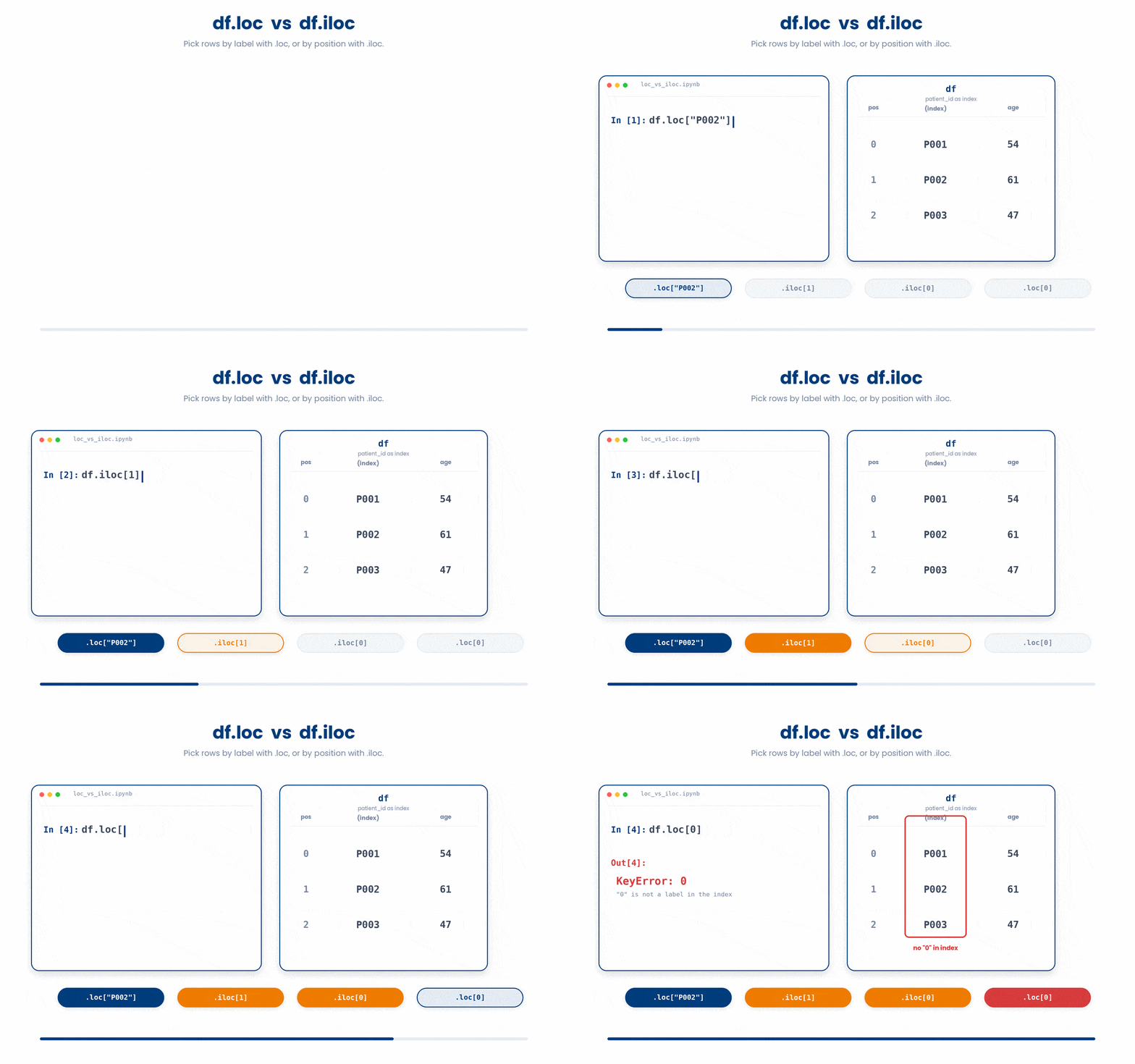
df.loc[2]gives you the row whose label is2df.iloc[2]gives you the third row by position (index).
For a DataFrame with the default 0, 1, 2, ... index, the two look identical. As soon as you set a meaningful index (patient_id, for instance), they diverge and the difference matters.
Rule of thumb: .loc is by name, .iloc is by number.
Try this snippet in the Python Scratchpad on the right.
import pandas as pd

df = pd.DataFrame(
    {"age": [54, 61, 47]},
    index=["P001", "P002", "P003"],
)

print(df.loc["P002"])
print(df.iloc[1])
print(df.iloc[0]).iloc also takes a slice, not just a single position: df.iloc[0:5] gives you the first five rows by position, exactly like slicing a list.
Both .iloc and .loc also take a second argument, separated by a comma — rows first, columns second, the same order as df.shape.
df.iloc[0:5, 0:3]picks the first five rows and the first three columns, by position.df.loc[df["age"] > 60, ["patient_id", "age", "bmi"]]picks every row whereageis over 60, keeping only thepatient_id,age, andbmicolumns, by condition and by name at the same time.
Try this snippet in the Python Scratchpad on the right.
import pandas as pd

df = pd.read_csv("patients.csv")
print(df.iloc[0:5])
print(df.iloc[0:5, 0:3])
print(df.loc[df["age"] > 60, ["patient_id", "age", "bmi"]])Rule of thumb: reach for the .loc form most often. It filters rows and picks columns in one readable step, instead of a filter followed by a separate column selection.
8.3 Boolean filtering
The most common thing you will ask is not "give me row three" but "give me every row where some condition is true." That is called boolean filtering, and it is the move you will reach for ten times a day.
Try this snippet in the Python Scratchpad on the right.
import pandas as pd

df = pd.DataFrame({
    "patient_id": ["P001", "P002", "P003", "P004"],
    "age": [54, 61, 47, 72],
    "bmi": [27.3, 24.1, 31.2, 22.8],
})
older = df[df["age"] > 60]
print(older)Read it in two steps:
df["age"] > 60produces aSeriesofTrueandFalse, one entry per row,Truewherever the condition holds.- Passing that
Seriesback intodf[...]keeps only the rows where the entry wasTrue.
Once your eye is trained for this pattern, you will read df[df["age"] > 60] without thinking.

8.4 Combining conditions
Use & for and, | for or, and put each condition in its own pair of round brackets. The brackets are not optional. & has higher precedence than the comparison operators, and without them Python parses the expression in a way that almost always raises an error.
Try this snippet in the Python Scratchpad on the right.
import numpy as np

arr = np.zeros(4)
print(arr)

arr = arr.reshape(2, 2)
print(arr)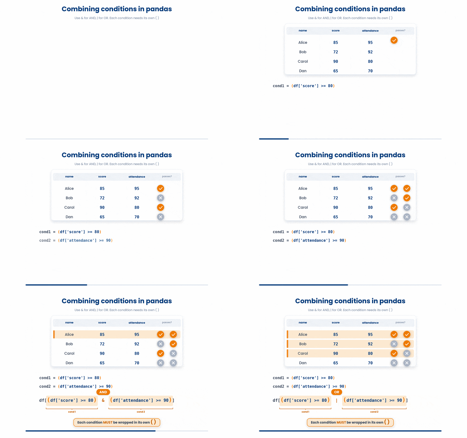
.query() is a second way to filter, where the whole condition is written as one string: df.query("age > 60 and bmi > 25") instead of df[(df["age"] > 60) & (df["bmi"] > 25)].
Try this snippet in the Python Scratchpad on the right.
import pandas as pd

df = pd.read_csv("patients.csv")
bracket = df[(df["age"] > 60) & (df["bmi"] > 25)]
query = df.query("age > 60 and bmi > 25")
print(bracket)
print(query)The two produce identical results. .query() reads more easily once conditions stack up: column names need no df[...] wrapper, and and / or are spelled as words instead of & / |, so the parentheses-around-every-condition rule from earlier stops applying.
It has one limit worth knowing: a column name containing a space needs backticks around it inside the query string, which is fiddly enough that people often rename the column instead. Bracket filtering has no such restriction and is still the form you will see most often in other people's code — treat .query() as a readable option, not a replacement.
8.5 Filtering by multiple categories with .isin
When you want every row whose clinic is one of "A", "B", or "C", you could write three conditions joined by | - but the cleaner way is .isin. Pass it a list of accepted values and it returns a boolean Series, True wherever the column value is in the list. Prefix with ~ to flip it ("not in"). This pairs perfectly with the boolean filtering pattern from earlier in this module.
Try this snippet in the Python Scratchpad on the right.
import pandas as pd

df = pd.DataFrame({
    "patient_id": ["P001", "P002", "P003", "P004", "P005"],
    "clinic": ["A", "B", "C", "D", "A"],
    "age": [54, 61, 47, 72, 38],
})

in_main_clinics = df[df["clinic"].isin(["A", "B", "C"])]
print(in_main_clinics)

elsewhere = df[~df["clinic"].isin(["A", "B", "C"])]
print(elsewhere)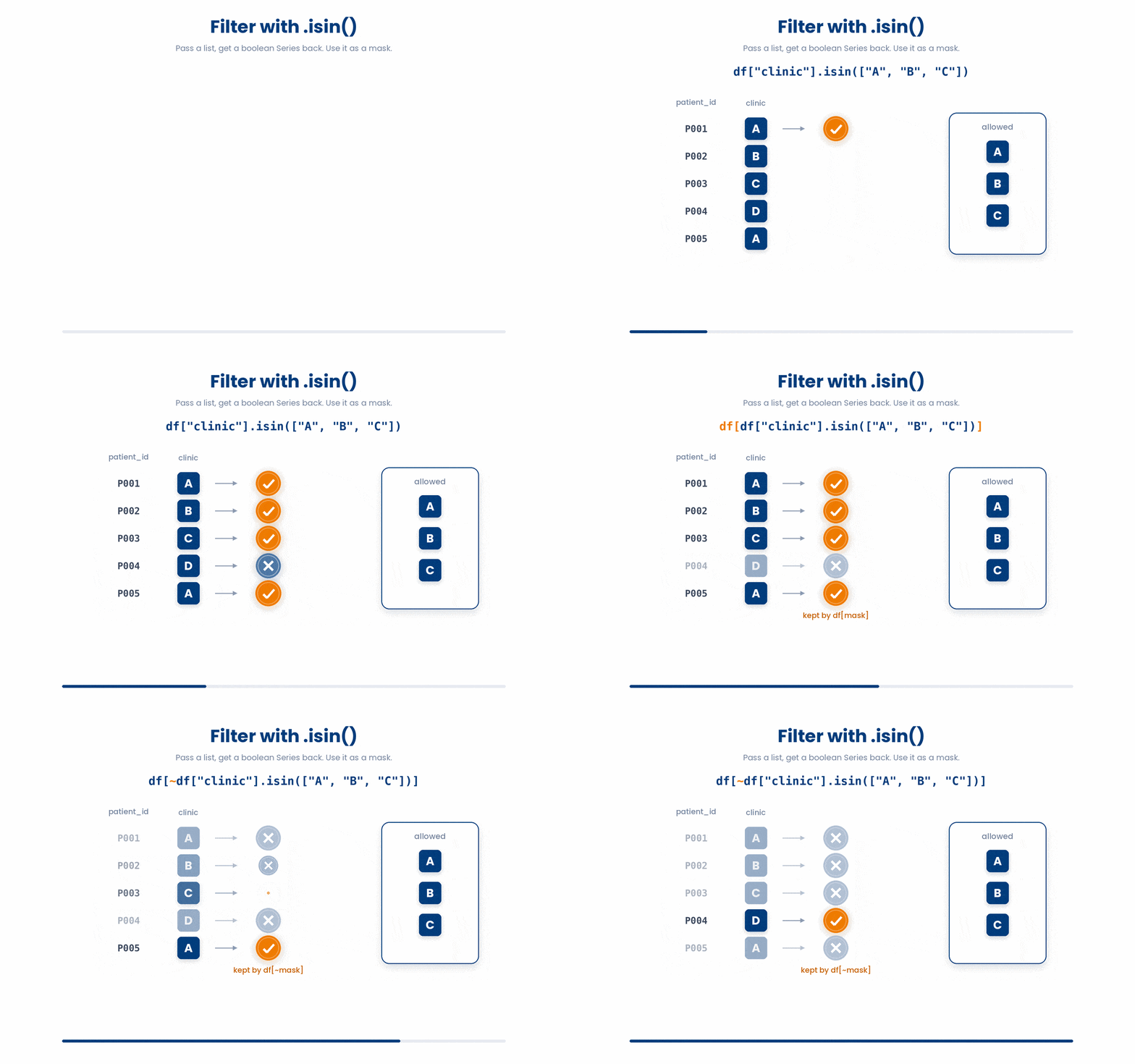
9 Putting it together
The seven tools in Part I are usually used together. A typical first pass on a new dataset reads the file, prints the shape and dtypes, looks at the first few rows, counts the categories of one column, parses any date columns, and filters down to the rows that matter for the question you are asking.
Work through this example in three stages. You unlock each stage only after the tutor confirms the previous one. Each stage removes more of the scaffolding — by the end you are writing it yourself.
Problem: You have patients.csv with columns patient_id, age, clinic, bmi, visit_date. Read it into a DataFrame, print its shape and info, count patients per clinic, parse visit_date as a date, and pull out the rows where age is over 60 and clinic is one of A, B, or C.
import pandas as pd

df = pd.read_csv("patients.csv")
print(df.shape)
print(df.info())
print(df["clinic"].value_counts())
df["visit_date"] = pd.to_datetime(df["visit_date"])
selected = df[(df["age"] > 60) & df["clinic"].isin(["A", "B", "C"])]
print(selected)- Load the CSV with pd.read_csv, then look at shape, info, and clinic counts so you know what you are working with before filtering.
- Convert visit_date with pd.to_datetime — until you do this it is just a string and any date arithmetic will silently misbehave.
- Build the filter as a boolean mask: each comparison needs parentheses because & has higher precedence than > or ==, and .isin() handles the "one of these values" check without chaining several ==.
The same solution with key parts replaced by ???.
Fill in every ??? so the code matches the reference,
then ask the tutor to check it.
Your turn: Build a DataFrame with five patients whose ages are 45, 67, 58, 72, 61 and whose clinics are A, B, A, C, D respectively. Print the number of patients aged over 60 whose clinic is A, B, or C.
10 Renaming columns and changing their type
Column names do not always arrive the way you would choose them. df.rename(columns={"chol": "cholesterol"}) relabels one or more columns by name — pass as many old-name-to-new-name pairs as you need in the one dictionary.
Like most pandas operations, rename returns a new DataFrame and leaves the original alone. Nothing changes unless you catch the result: df = df.rename(columns={...}).
Try this snippet in the Python Scratchpad on the right.
import pandas as pd

df = pd.read_csv("patients.csv")
df = df.rename(columns={"chol": "cholesterol", "bmi": "body_mass_index"})
print(df.columns)Renaming forty columns one pair at a time is exactly the kind of typing pandas is meant to save you from. Assign a whole list straight to df.columns instead, and every column is relabelled at once.
Build that list the way you built a column selection earlier in this part — a comprehension over the names you already have. [c.replace("lab_", "") for c in df.columns] strips a lab_ prefix off every column name.
Try this snippet in the Python Scratchpad on the right.
import pandas as pd

df = pd.DataFrame({
    "lab_glucose": [95, 110, 88],
    "lab_hba1c": [5.4, 6.1, 5.0],
    "patient_id": ["P001", "P002", "P003"],
})
df.columns = [c.replace("lab_", "") for c in df.columns]
print(df.columns)Be careful with this form. The new list is positional and must be exactly as long as the number of columns you have — item one becomes the new name of column one, and so on. Get the order or the length wrong and every value is silently mislabelled, with no error to warn you.
.astype() changes a column's dtype outright. df["age"].astype("float64") converts a whole-number column to decimal. Going the other way truncates towards zero rather than rounding, so converting 27.9 to an integer type gives 27, not 28.
Try this snippet in the Python Scratchpad on the right.
import pandas as pd

df = pd.DataFrame({"age": [54, 61, 47]})
print(df["age"].dtype)
print(df["age"].astype("float64"))

bmi = pd.Series([27.9, 24.1, 31.6])
print(bmi.astype("int64"))The commonest real use of .astype() is converting a column to the category dtype. A column like sex, clinic, or diagnosis holds a small set of labels that repeat over and over. Storing it as category keeps one copy of each label and a compact code per row, instead of repeating the full string every time.
This is not only about memory, though on a large table it saves plenty. It tells pandas — and the plotting libraries later in this course — that the column is a set of groups, not free text.
Try this snippet in the Python Scratchpad on the right.
import pandas as pd

df = pd.read_csv("patients.csv")
print(df.dtypes)
df["clinic"] = df["clinic"].astype("category")
print(df.dtypes)
print(df["clinic"].cat.categories)select_dtypes picks columns by type instead of by name. df.select_dtypes(include=["number"]) returns every numeric column at once; df.select_dtypes(include=["category", "object"]) returns the label columns instead.
Try this snippet in the Python Scratchpad on the right.
import pandas as pd

df = pd.read_csv("patients.csv")
numeric_only = df.select_dtypes(include=["number"])
labels_only = df.select_dtypes(include=["category", "object"])
print(numeric_only.columns)
print(labels_only.columns)Machine-learning code almost always wants that numeric block on its own — most models cannot take a text column as input at all — so select_dtypes(include=["number"]) is usually the first line of preparing a table for one.
Six dtypes cover almost everything you will meet in this course:
int64— whole numbers.float64— decimal numbers.object— text, and anything elsepandashas no more specific type for.category— a column of repeated labels, stored compactly.bool—True/False.datetime64[ns]— the typepd.to_datetimeproduces.
11 Check your understanding
You have reached the end of the module. Try the same questions again — your answers here, paired with your pre-test answers, are how we measure what the module taught you. Answer every question and confidence rating, then click Submit and see results to view your score.
You write df = pd.DataFrame({"a": [1, 2, 3], "b": [10, 20, 30]}). What does df["a"] return?
Which of these reads a tab-separated file into a DataFrame?
A column of strings like "2024-01-15" is in your DataFrame. After running df["d"] = pd.to_datetime(df["d"]), what dtype does d have?
Which call reports the dtype and the number of non-null values for every column of df?
df["clinic"].value_counts() returns which kind of object?
A DataFrame is indexed by patient_id ("P001", "P002", "P003", ...). Which call returns the row for patient "P002"?
You want every row in df where age > 50 AND bmi > 25. Which expression is correct?
You want every row whose clinic is one of "A", "B", or "C". Which expression works?
I can read a CSV or Excel file into a DataFrame and use head, info, and describe to get a quick feel for what is in it.
I can filter a DataFrame on one or more boolean conditions and pull out the rows that match.
I can parse a column of date strings with pd.to_datetime and pull out the year or month with .dt.
12 Your results
Here is how your post-test answers compare with your pre-test answers. The pre/post pairing is the most reliable way to see what this module actually taught you.
Submit the post-test to see your results.
What is the one thing from this module that is still unclear to you?