

1 Before you start
This is not graded, and it does not count towards anything. Answer every question even if you are only guessing — having a go at something before you have been taught it is one of the best ways to remember it afterwards. The lesson ends with another short check, and there you will be shown the correct answer for anything you missed. Choose an option for every question and confidence rating, then click Submit answers.
What happens when you write arr.shape() with parentheses, on a NumPy array?
What is the dtype of np.array([54, 61, 72.5])?
What does np.arange(0, 10, 2) produce?
You have arr = np.array([1, 2, 3, 4]). What does arr * 2 produce?
What does np.sqrt(np.array([1, 4, 9, 16])) return?
For ages = np.array([54, 61, 47, 72, 38]), what does ages[1:4] return?
You have a 2D array m with shape (3, 4). What does m[:, 0] return?
For ages = np.array([54, 61, 47, 72, 38]), what shape does ages.reshape(-1, 1) give?
I can build a NumPy array from a Python list and read its shape, dtype, and size attributes.
I can do element-wise arithmetic on a NumPy array, index single values and slices of a 1D or 2D array, and reshape an array into a different shape.
2 Introduction
While standard Python lists are great for basic data storage, they struggle with heavy numerical work. If you want to modify a list of 1,000 patient ages or find their average, standard Python requires writing slow loops or using extra modules step-by-step.
NumPy is the package that solves this. While a NumPy array looks like a standard Python list on the outside, underneath it is a tightly packed data grid designed specifically for high-speed math.
Instead of writing clunky loops and multiple lines of code, NumPy lets you perform heavy calculations with a single expression. With just one line, you can add five to every age, multiply entire datasets together, calculate the average of a million numbers, or instantly filter for patients over 65.
This first part of the NumPy module covers the foundations you reach for before any analysis:
- Introduction to NumPy arrays - what an array is, how to create one, and the three attributes (shape, dtype, size) that describe it.
- Array operations and indexing - element-wise arithmetic, picking out single values or slices, and the way 2D arrays use a row, column index.
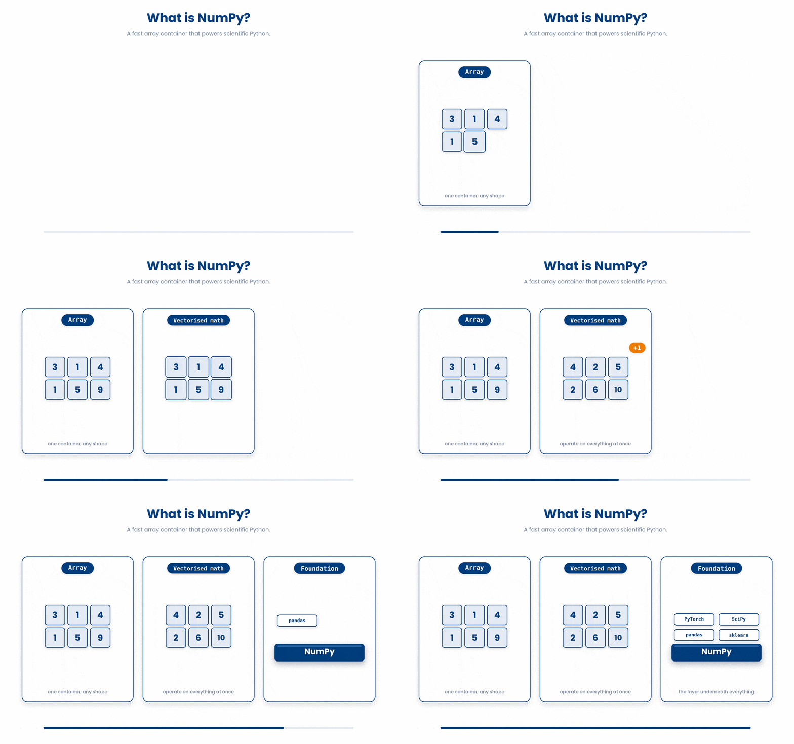
Try every snippet in the Python Scratchpad on the right. By the end of this part you will build NumPy arrays from data, perform vectorised arithmetic, and index 1D and 2D arrays with positions and slices.
3 Introduction to NumPy arrays
NumPy is a third-party package, so the first step is to make it available to your script. The convention is to import it under the alias np. From that point on, every NumPy tool is reached as np.something.
Try this snippet in the Python Scratchpad on the right.
import numpy as np
ages = np.array([54, 61, 47, 72, 38])
print(ages)np.array takes a regular Python list and turns it into a NumPy array. When you print the result, you will see something that looks like a list with no commas: [54 61 47 72 38]. That spacing is NumPy's way of showing you the value is an array, not a list. From here on you can do array things to it - add a number to every element, take the mean, slice it - in a way you cannot do to a plain list.
Every NumPy array carries three pieces of information about itself that you can read with the dot syntax:
shape- a tuple describing how many elements there are along each dimension. For a 1D array of five numbers, the shape is(5,). The trailing comma is Python's way of writing a one-element tuple.dtype- the type of value inside the array. All elements of a NumPy array share the same type, sodtypeis one value, not a list. Common ones areint64(whole numbers),float64(decimals), andbool.size- the total number of elements. For a 1D array this is the same aslen(arr).
Try this snippet in the Python Scratchpad on the right.
import numpy as np
weights = np.array([72.5, 68.0, 80.2, 65.4])
print(weights.shape)
print(weights.dtype)
print(weights.size)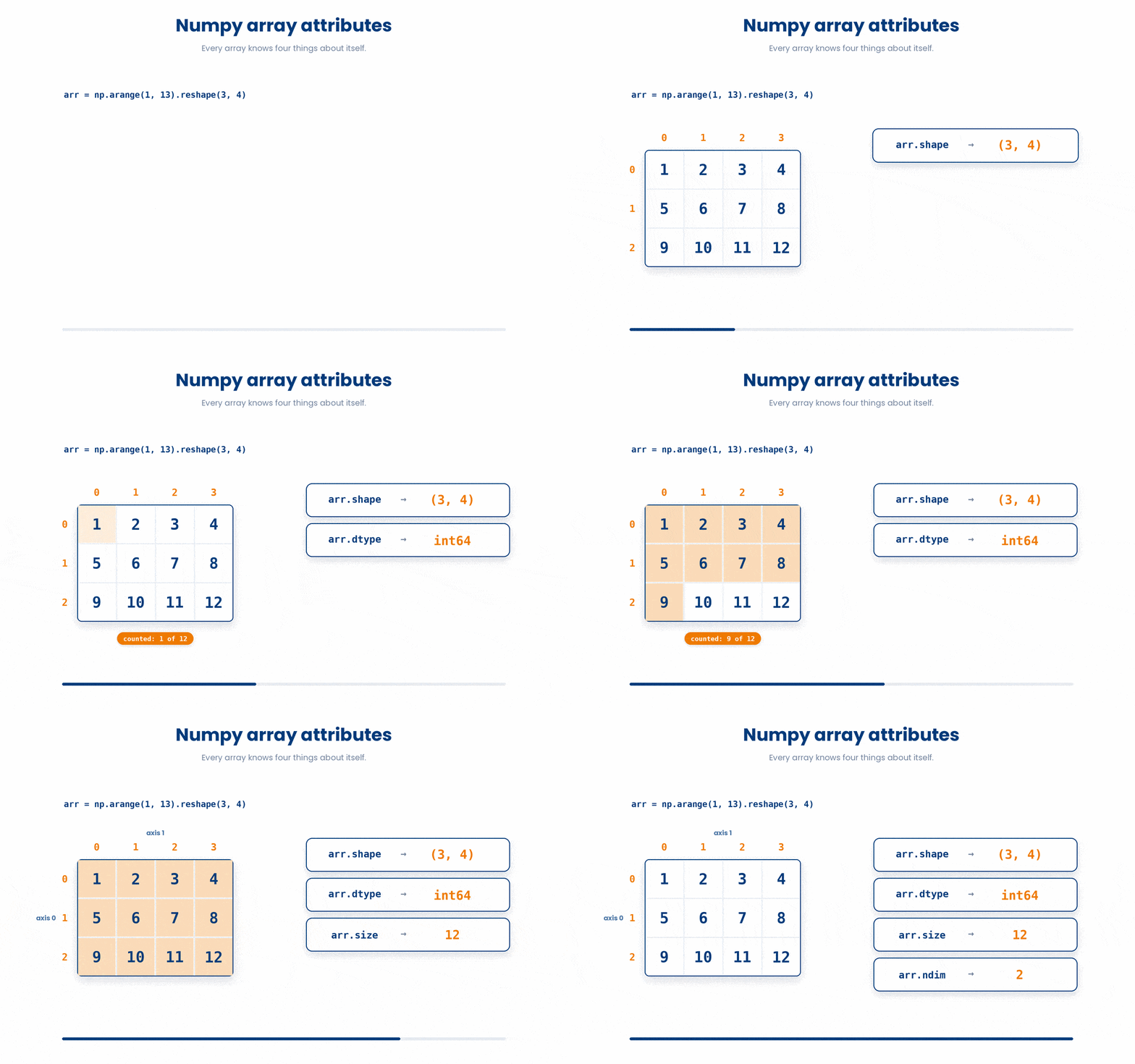
Notice that shape, dtype, and size do not have round brackets after them.
This is because shape, dtype, and size are attributes (stored data) rather than methods (functions), they don't take round brackets. Writing weights.shape() is a classic beginner mistake that will cause Python to throw a "tuple object is not callable" error.
Read the code carefully and type what you think it will print. Click Submit prediction for AI tutor feedback comparing your prediction against the real output, then click Reveal actual output to run the snippet yourself and see what happens.
import numpy as np
ages = np.array([54, 61, 47, 72, 38])
print(ages.size)Every array you have built so far picked its own dtype: whole numbers became int64, decimals became float64. You do not have to accept that choice. Pass a dtype keyword when you create the array and NumPy stores every element in that type instead.
int8,int16,int32,int64- whole numbers stored in 8, 16, 32, or 64 bits. The number is the size of the box:int8only holds -128 to 127, whileint64stretches to roughly plus or minus 9.2 quintillion. Each has an unsigned version too, such asuint8, which drops the negative half and uses that space to reach further in the positive direction instead - 0 to 255.float32,float64- decimals stored in 32 or 64 bits.float64is what NumPy uses by default and keeps about 15 to 17 significant digits;float32keeps about 7, which is fine for most measurements but rounds off sooner.
Try this snippet in the Python Scratchpad on the right.
import numpy as np
small = np.array([10, 20, 30], dtype=np.int8)
big = np.array([10, 20, 30], dtype=np.int64)
print(small.dtype, small.itemsize)
print(big.dtype, big.itemsize)
precise = np.array([1 / 3], dtype=np.float64)
rounded = np.array([1 / 3], dtype=np.float32)
print(precise)
print(rounded)itemsize reports how many bytes one element takes - 1 for int8, 8 for int64 - matching the bit counts in their names, since a byte is 8 bits. Look at the last digit of precise versus rounded: the same fraction, one third, prints differently because float32 ran out of room to store it exactly.
dtype only works at creation time. To change the type of an array you already have, use .astype(). It returns a new array with every element converted, leaving the original alone - the same non-destructive habit as .reshape().
Widen a type when an operation demands it. Try to divide an integer array in place - arr /= 2 - and NumPy refuses outright with a casting error, because the true answer needs decimals and an integer array has nowhere to put them. Converting to float64 first is the fix:
Try this snippet in the Python Scratchpad on the right.
import numpy as np
scores = np.array([1, 2, 3], dtype=np.int32)
converted = scores.astype(np.float64)
print(converted, converted.dtype)Narrow a type the other way when you know the range is small and want to save memory - an image's pixel values never leave 0-255, so storing them as uint8 uses a quarter of the space int32 would. But narrowing has a cost NumPy never warns you about: a value that does not fit the target type wraps around instead of raising an error, and converting a decimal to an integer truncates it rather than rounding it.
Try this snippet in the Python Scratchpad on the right.
import numpy as np
counts = np.array([120, 125, 130, 200])
prices = np.array([19.99, 4.5, 100.1])
print(counts.astype(np.int8))
print(prices.astype(np.int32))counts.astype(np.int8) turns 130 into -126 and 200 into -56, each one wrapped past int8's ceiling of 127 and continuing from the bottom. prices.astype(np.int32) drops every decimal place outright: 19.99 becomes 19, not 20, and 4.5 becomes 4, not 5. Rule of thumb: only narrow a dtype when you are certain of the range, and call np.round() before converting to int if you actually want the nearest whole number rather than the truncated one.
So far we have built arrays from a list we typed in. NumPy also gives you a few constructors for making arrays without typing the values one by one. These come up constantly when you need a block of placeholder values to fill in later, or a regular sequence of numbers for an axis of a plot.
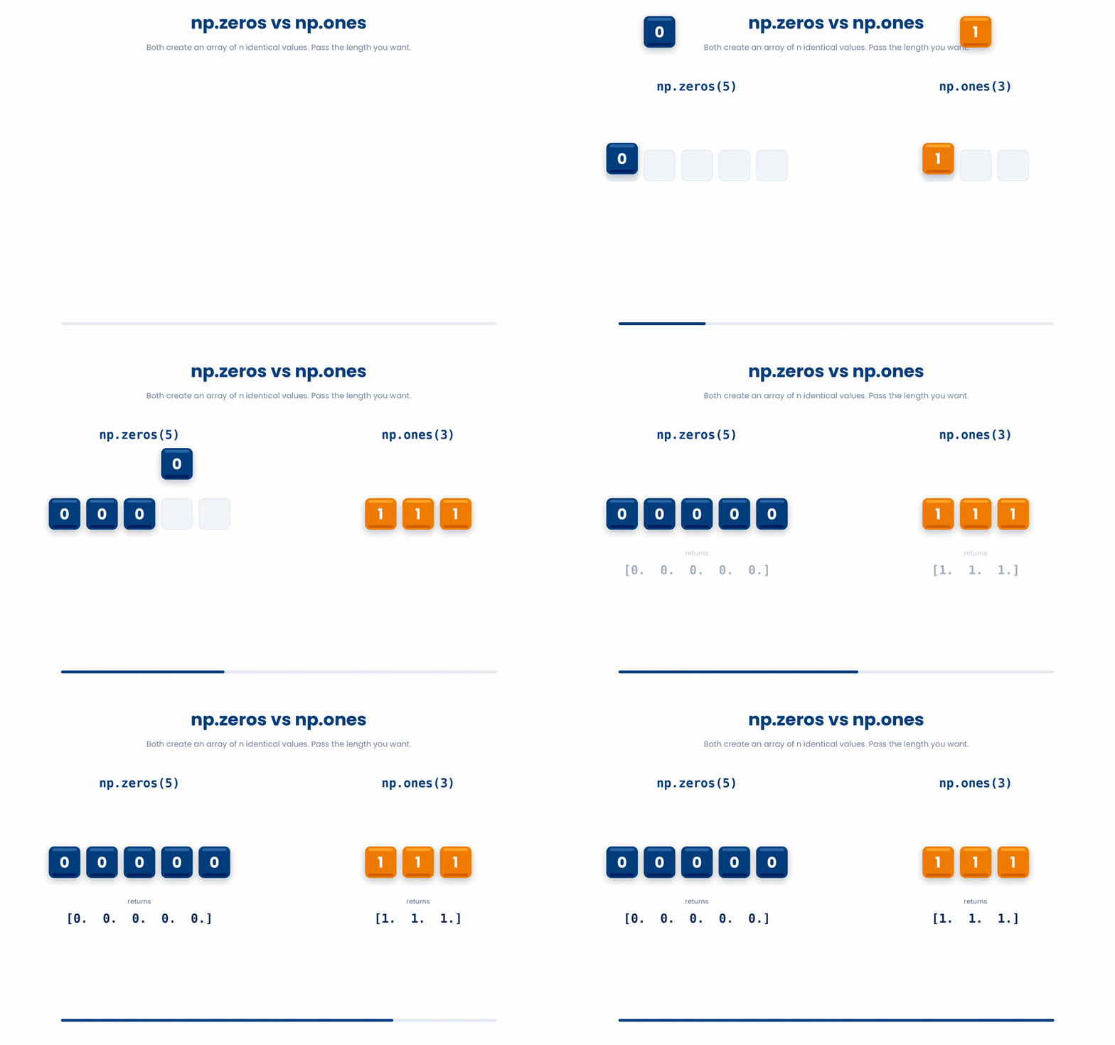
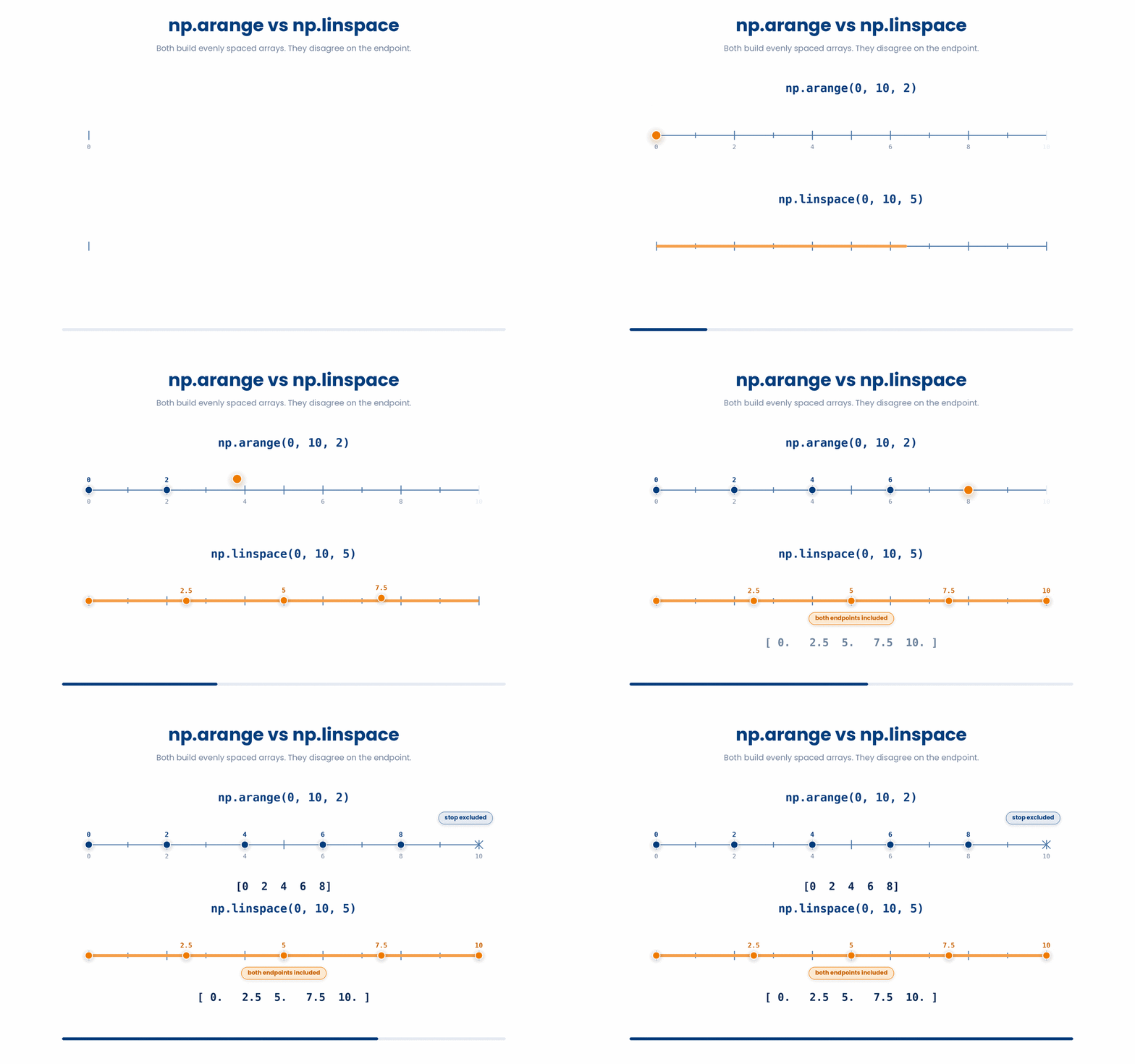
np.zeros(n)- an array ofnzeros.np.zeros(5)is[0. 0. 0. 0. 0.].np.ones(n)- an array ofnones.np.ones(3)is[1. 1. 1.].np.arange(start, stop, step)- like Python's built-inrange, but it returns an array.np.arange(0, 10, 2)is[0 2 4 6 8].np.linspace(start, stop, n)-nevenly spaced values fromstarttostop, both ends included.np.linspace(0, 1, 5)is[0. 0.25 0.5 0.75 1. ].
- Here is an image to illustrate
np.zerosandnp.ones
- …and
np.arangeandnp.linspace.
- Try the following to see these functions in action:
Try this snippet in the Python Scratchpad on the right.
import numpy as np

print(np.zeros(4))
print(np.ones(3))
print(np.arange(0, 10, 2))
print(np.linspace(0, 1, 5))4 Random number generation with np.random
Many data analyses rely on random numbers for tasks like generating fake datasets, shuffling rows, or sampling patients. To handle this, use NumPy's np.random module.
The modern best practice is to create a random number generator using np.random.default_rng(seed). Setting a "seed" makes your output reproducible so that your code will produce the exact same sequence of "random" numbers every time it runs. This is a crucial step to ensure you can repeat your analysis. Try it out!
Try this snippet in the Python Scratchpad on the right.
import numpy as np
rng = np.random.default_rng(seed=42)
ages = rng.integers(20, 90, size=10)
print(ages)
shuffled = rng.permutation(ages)
print(shuffled)
You will also run into an older style of doing this: np.random.seed(0) followed by calls like np.random.random(5). It is the same idea as default_rng - fix a seed, get the same numbers back every run - through one global generator shared across your whole program, rather than a generator you create and hold in a variable yourself. You do not need to switch to it; just recognise it as the same idea when you meet it in someone else's code or in older documentation.
5 2D or 3D NumPy arrays
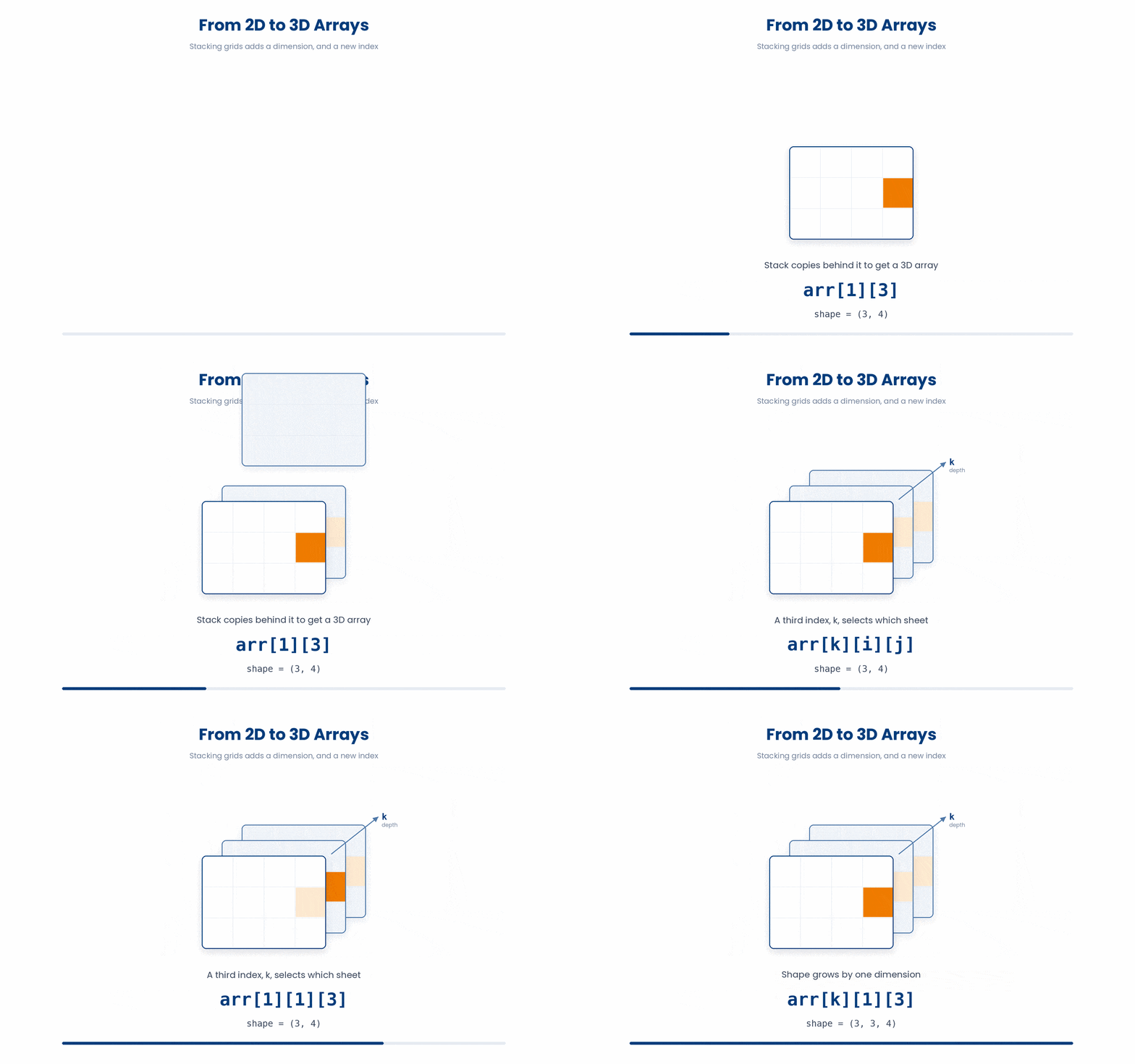
Arrays are not limited to one dimension. A 2D array is a grid of values - rows and columns - which is exactly the shape your data takes when you have several measurements per patient. You build a 2D array from a list of lists, where each inner list becomes a row.
Try this snippet in the Python Scratchpad on the right.
import numpy as np
patients = np.array([
    [54, 72.5, 1.75],
    [61, 68.0, 1.80],
    [47, 80.2, 1.68]
])
print(patients)
print(patients.shape)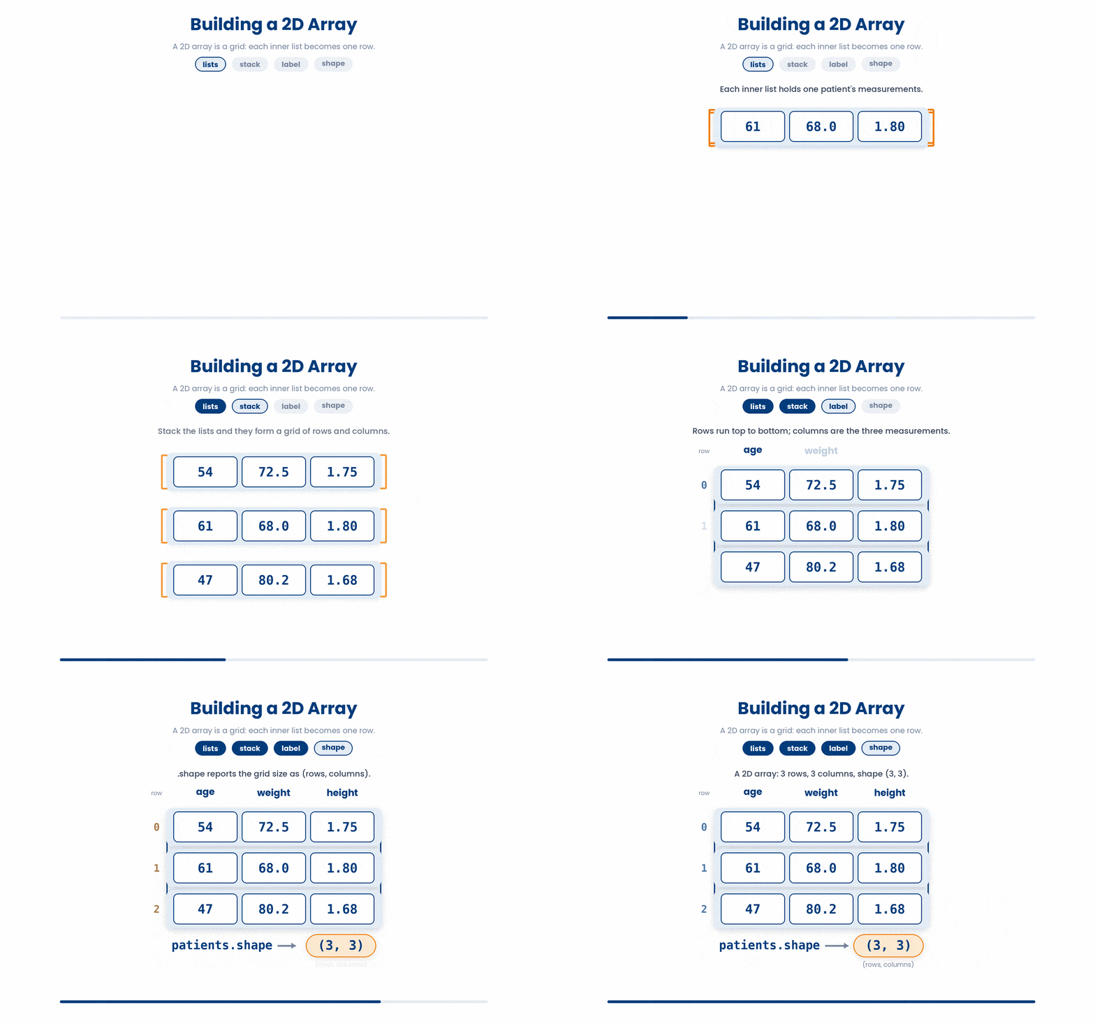
The shape of this array is (3, 3) - three rows, three columns. When you print it, NumPy lays it out as a grid so you can read the rows and columns at a glance. Notice that even though the ages were whole numbers, NumPy has shown them as 54., 61., 47. with a trailing dot. That is because every element of an array shares one dtype, and once a single float (like 72.5) sits in the data, NumPy promotes the whole array to float64.
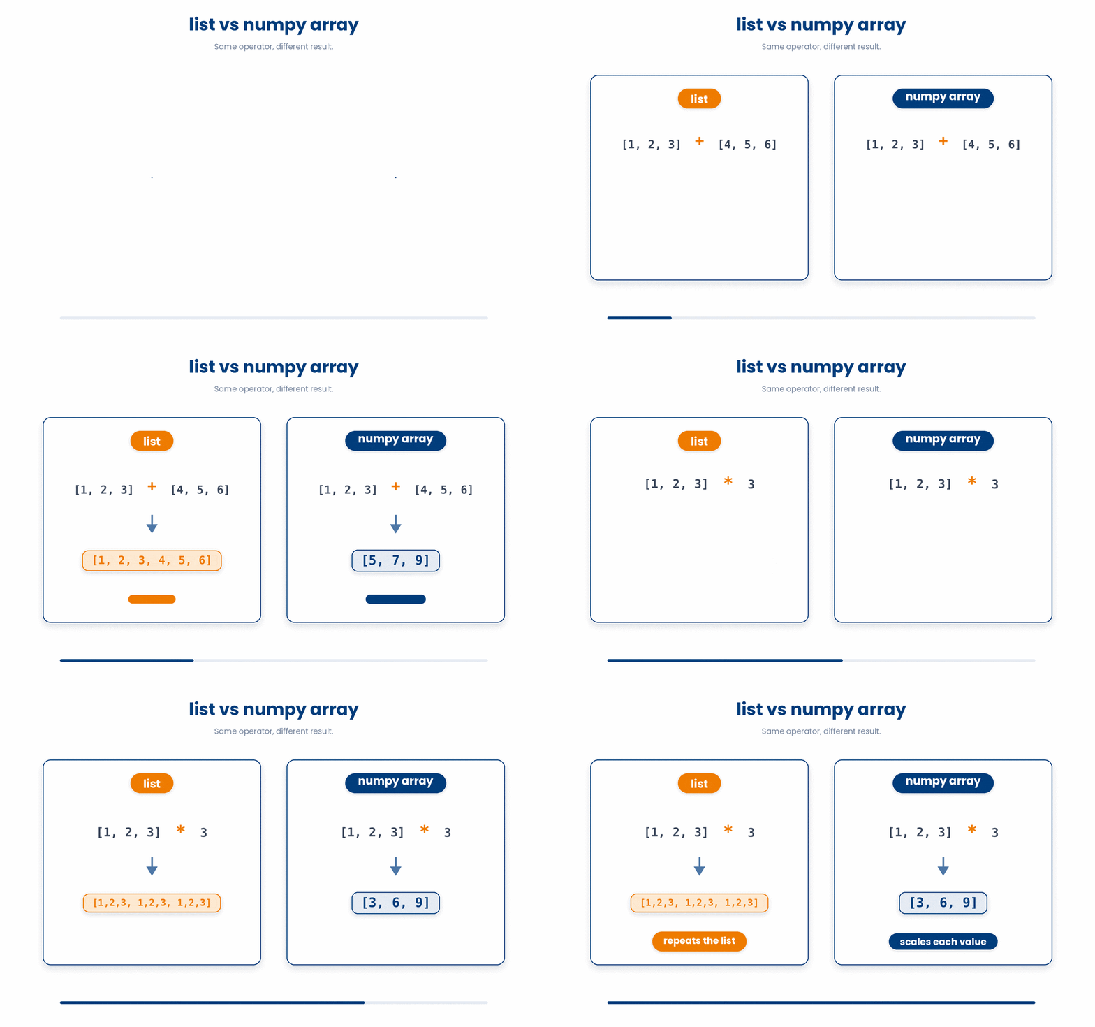
One final, crucial point: while NumPy arrays and Python lists look similar, they have very different rules.
Here is what you need to remember:
- Data Types: A Python list can hold a mix of anything (a string, an integer, and another list all together). A NumPy array is strict—every element must be the exact same type (a shared dtype).
- Growing Data: A list can easily grow as you append new items. An array has a fixed size. To make it bigger, you actually have to build a brand-new, larger array.
- Extensive Operations: The powerful tools we will cover next—like instant math, fast statistics, and simple filtering—only work on arrays, not lists.
6 Array broadcasting and operations
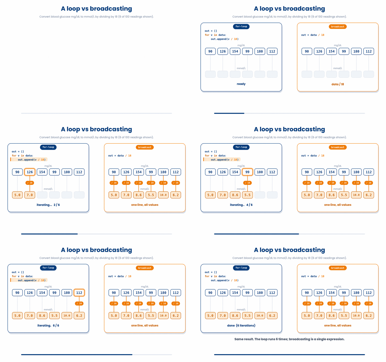
Imagine you have an array of blood glucose readings from a hundred patients, and you need to convert each one from mg/dL to mmol/L (dividing by 18).
With a plain Python list, you would write a loop: step through each value, divide it, append it to a new list. Slow and verbose.
NumPy's shortcut is broadcasting. Instead of looping, you write a single expression for the entire array. When you divide the array by 18, NumPy "broadcasts" that lone number across every position so the mathematical shapes line up, converting all 100 readings instantly.
6.1 Element-wise arithmetic
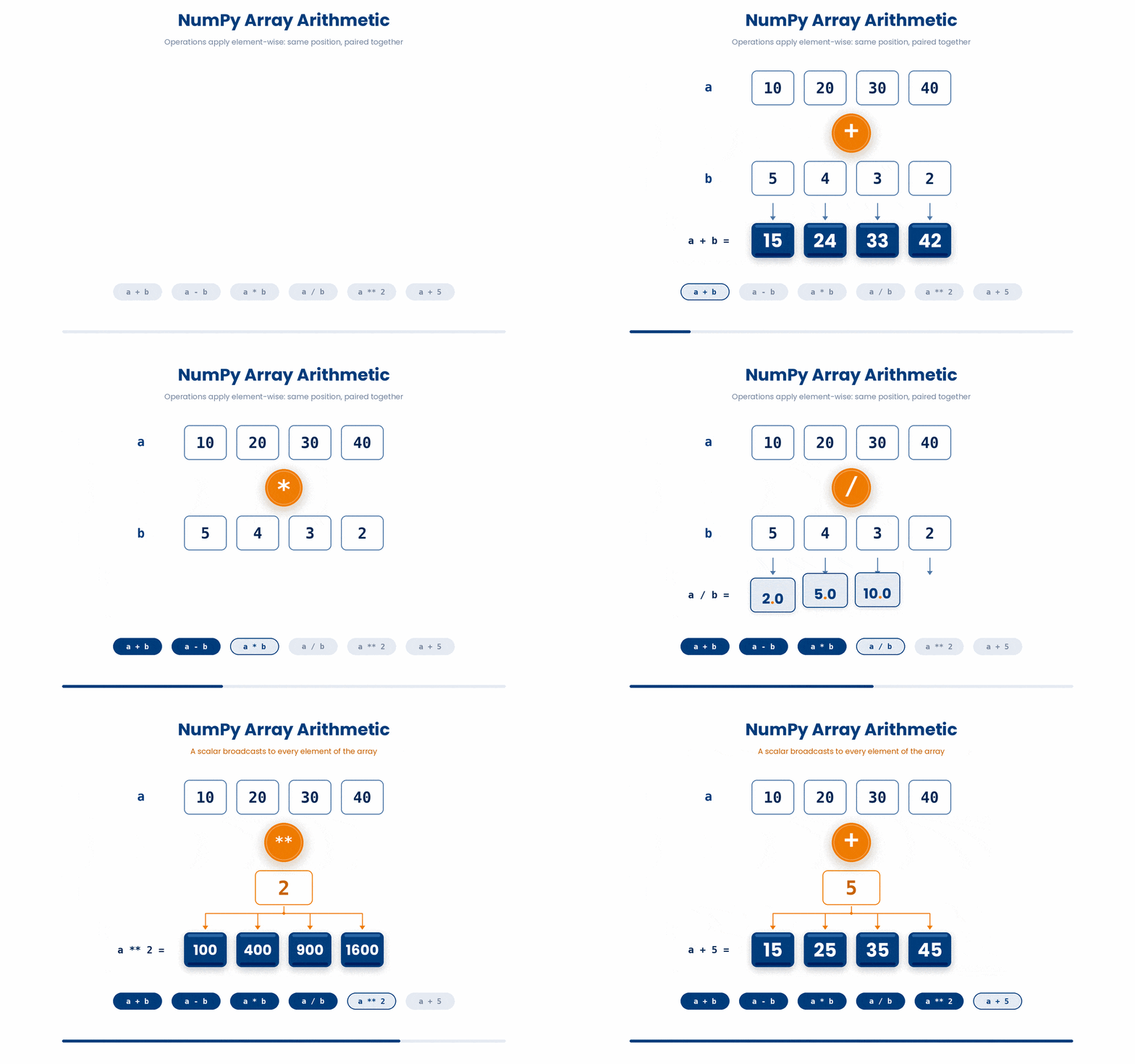
The first big payoff of using NumPy is element-wise arithmetic. Add a number to an array and the addition happens once for every element, with no loop in sight. The same is true for subtraction, multiplication, division, and exponentiation.
Try this snippet in the Python Scratchpad on the right.
import numpy as np
ages = np.array([54, 61, 47, 72, 38])
print(ages + 5)
print(ages * 2)When you write ages + 5, NumPy instantly creates a brand-new array where 5 is added to every single element (leaving you with [59, 66, 52, 77, 43]). Don't worry—your original ages array is left completely untouched! Similarly, typing ages * 2 simply doubles every number.
Broadcasting takes that single number (like the 5) and "broadcasts" it across every position in your array.
The best part? You didn't have to write a single for loop to make this happen. Behind the scenes, NumPy runs all of this using fast, compiled code. If you were working with a dataset of a million values, this method would be significantly faster than running a manual loop on a standard Python list.
Two more operators work the same elementwise way: // (floor division) and % (modulo, the remainder after dividing). You already used both on single numbers - point either one at an array instead and NumPy applies it to every element at once, exactly like + and * above.
Try this snippet in the Python Scratchpad on the right.
import numpy as np
ages = np.array([54, 61, 47, 72, 38])
print(ages // 10)
print(ages % 10)Every example so far - // 10 and % 10 included - has combined an array with a single number. NumPy will just as happily combine two arrays of the same length: it lines them up position by position and applies the operator to each pair, the first element of one with the first element of the other, the second with the second, and so on. The two arrays must be the same length, or NumPy raises an error rather than guessing what you meant.
Try this snippet in the Python Scratchpad on the right.
import numpy as np
before = np.array([148, 152, 139, 161, 144])
after = np.array([136, 140, 130, 142, 133])
change = after - before
print(change)change[0] is after[0] - before[0], change[1] is after[1] - before[1], and so on - five independent subtractions computed in one expression, with no loop and no indexing required.
Try this snippet in the Python Scratchpad on the right.
import numpy as np
weights = np.array([72.5, 68.0, 80.2])
heights = np.array([1.75, 1.80, 1.68])
bmi = weights / (heights ** 2)
print(bmi)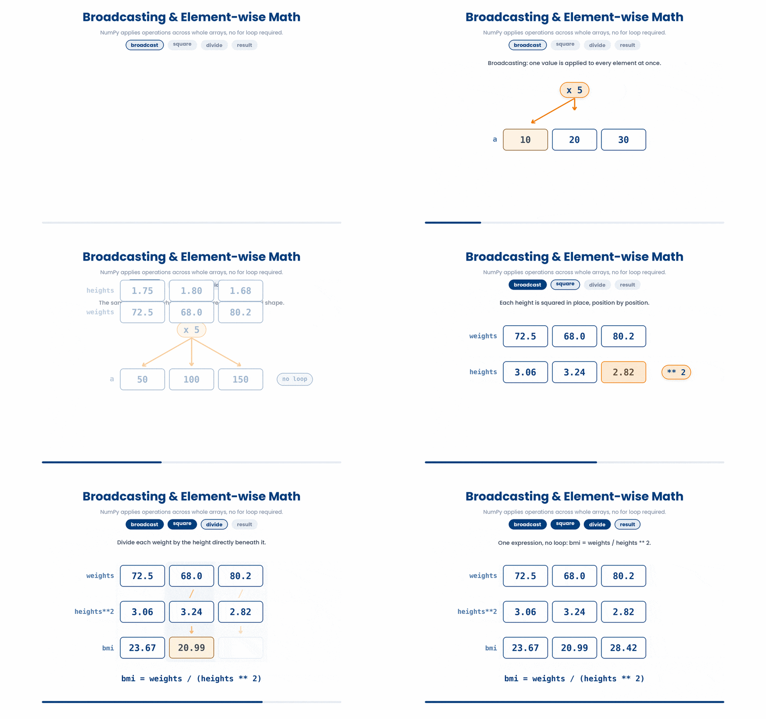
6.2 Broadcasting beyond arithmetic
You've already seen that adding a single number to an array adds it to every element. The same idea extends to two arrays, as long as their shapes are compatible.
Take a (5, 3) array of patient measurements: five patients down the rows, three variables across the columns. The mean of each column gives you a row of three values, shape (3,). Subtracting that row from the full array centres every column in one expression, because NumPy lines the two shapes up from the right and stretches the single row down all five rows.
The general rule is that two arrays can broadcast when each pair of dimensions is either equal or one of them is 1.
Try this snippet in the Python Scratchpad on the right.
import numpy as np
patients = np.array([
    [54, 72.5, 1.75],
    [61, 68.0, 1.68],
    [47, 80.2, 1.82],
])
column_means = patients.mean(axis=0)
print(column_means)
centred = patients - column_means
print(centred)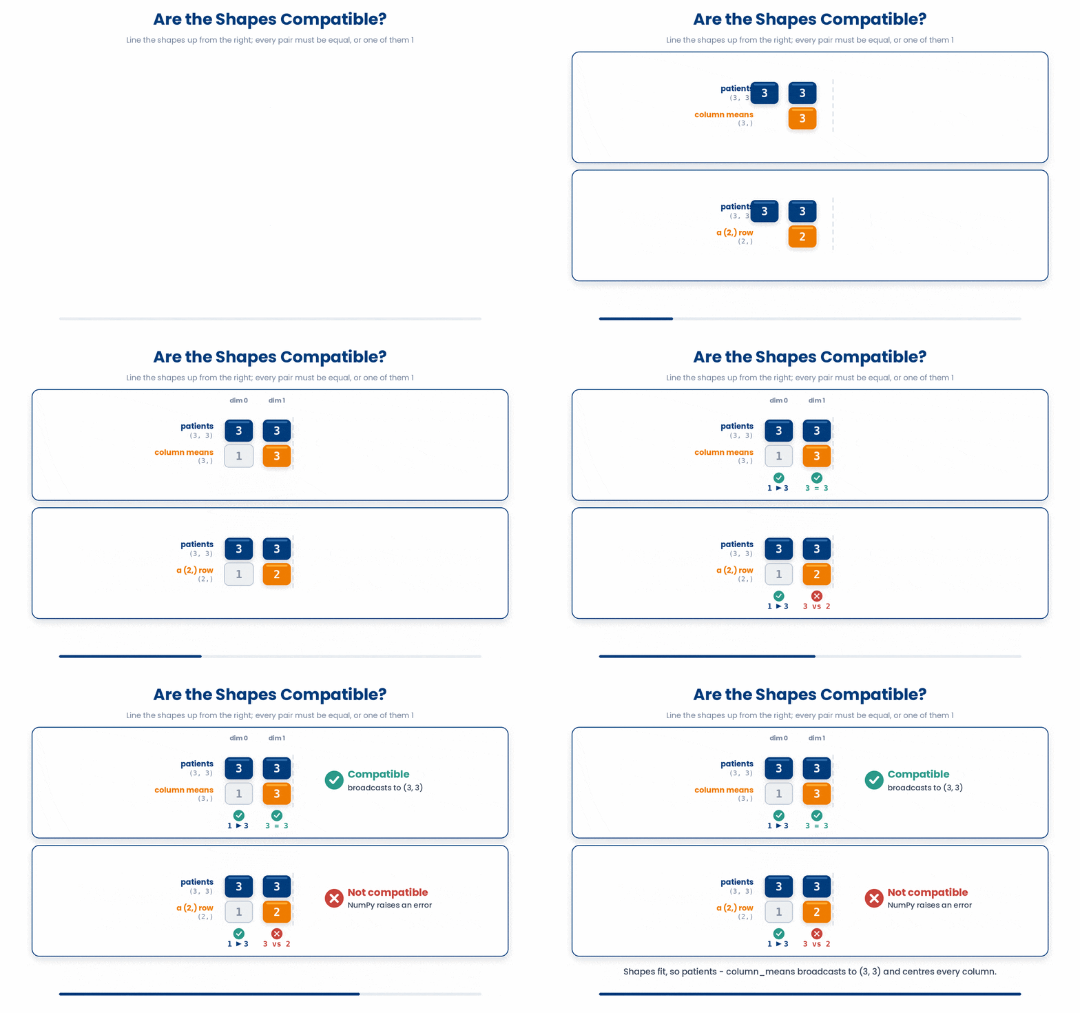
NumPy also gives you a stack of mathematical functions that behave the same way - apply once to the whole array, return a new array of the same shape. np.sqrt, np.log, np.exp, and np.abs are the ones you will meet first. Each one runs the function on every element.
Try this snippet in the Python Scratchpad on the right.
import numpy as np
values = np.array([1, 4, 9, 16, 25])
print(np.sqrt(values))6.3 Math functions: np.log and np.exp
Alongside np.sqrt you will often reach for np.log (natural logarithm) and np.exp (e raised to a power). Both behave element-wise like every other NumPy function - one call works on the whole array. They show up whenever you transform skewed lab values to a more symmetric scale (log-transform), or convert a log-odds back to a probability.
Try this snippet in the Python Scratchpad on the right.
import numpy as np
values = np.array([1, 10, 100, 1000])
print(np.log(values))
print(np.exp([0, 1, 2]))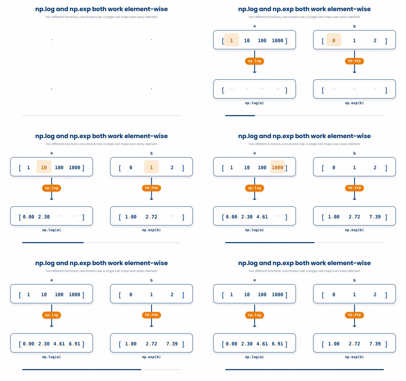
7 Array indexing
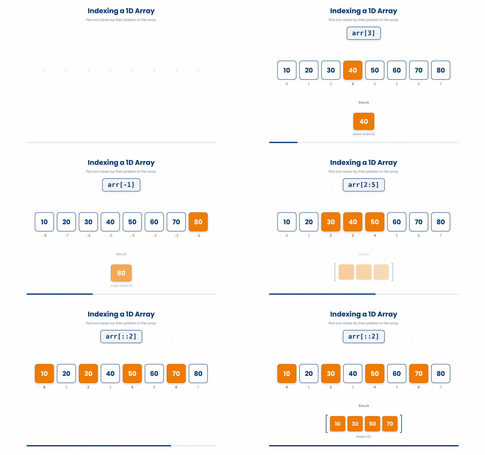
Pulling a single value out of a 1D array uses the same square-bracket syntax as a list. The first element is at index 0, the last at index -1. A slice arr[a:b] gives you a smaller array from index a up to but not including b - the same rule lists follow.
Try this snippet in the Python Scratchpad on the right.
import numpy as np
ages = np.array([54, 61, 47, 72, 38])
print(ages[0])
print(ages[-1])
print(ages[1:4])ages[0] is 54, the first element. ages[-1] is 38, the last. ages[1:4] is the slice [61 47 72] - elements at indices 1, 2, and 3 (4 is excluded). A slice of an array is itself a NumPy array, so all the same operations are available on it.
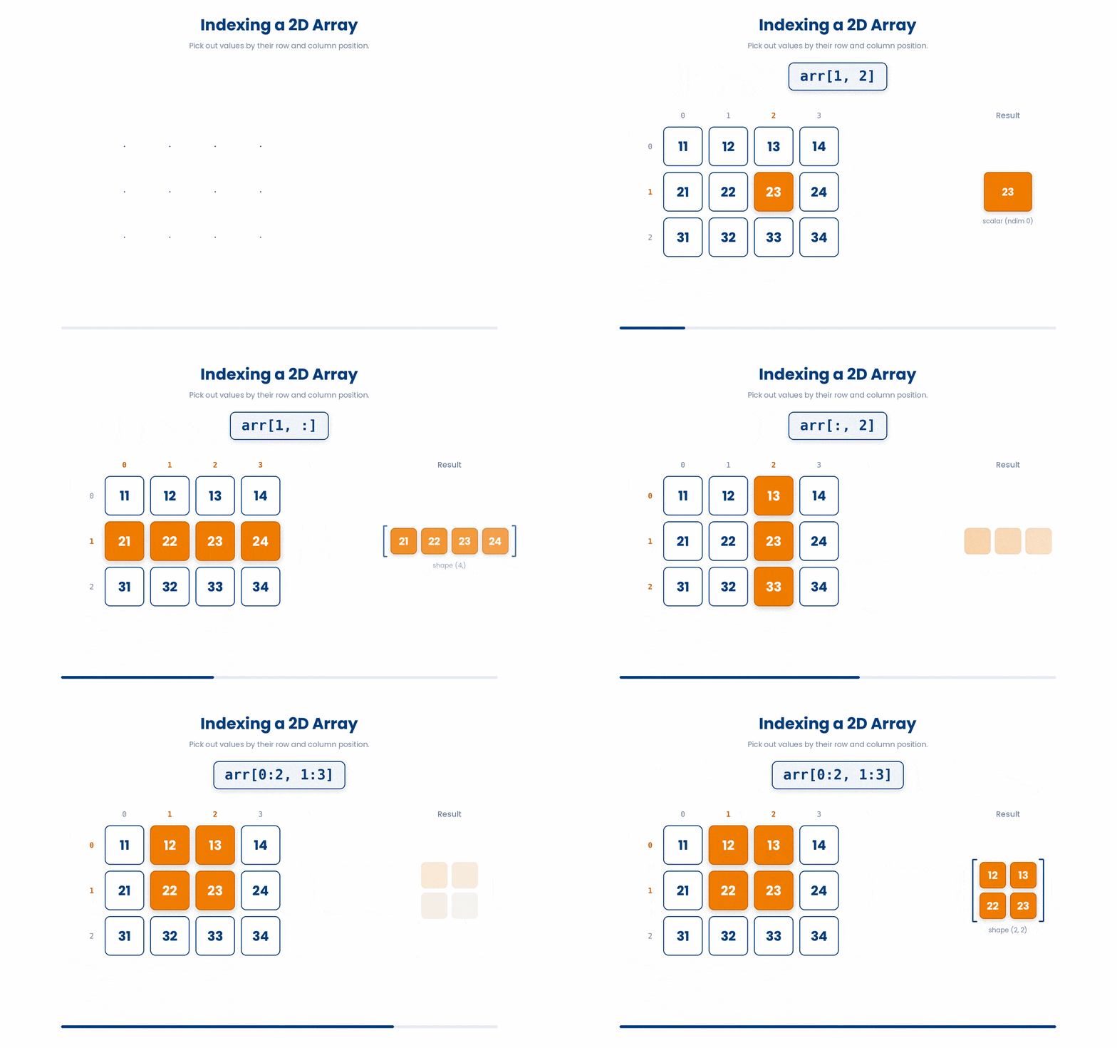
For 2D arrays the indexing is slightly richer because you have two axes to address. The shape is (rows, columns) and the indexing follows the same order: arr[row, column]. A colon on either side means "all of that axis".
Try this snippet in the Python Scratchpad on the right.
import numpy as np
patients = np.array([
    [54, 72.5, 1.75],
    [61, 68.0, 1.80],
    [47, 80.2, 1.68]
])
print(patients[0, 1])
print(patients[0, :])
print(patients[:, 0])patients[0, 1] is the value in row 0, column 1 - the weight of the first patient, 72.5. patients[0, :] is the whole first row - all three values for the first patient. patients[:, 0] is the whole first column - the ages of all three patients. Once you have data in this shape, the colon trick is how you ask questions like "give me every patient's BMI" or "give me the third measurement for every patient."
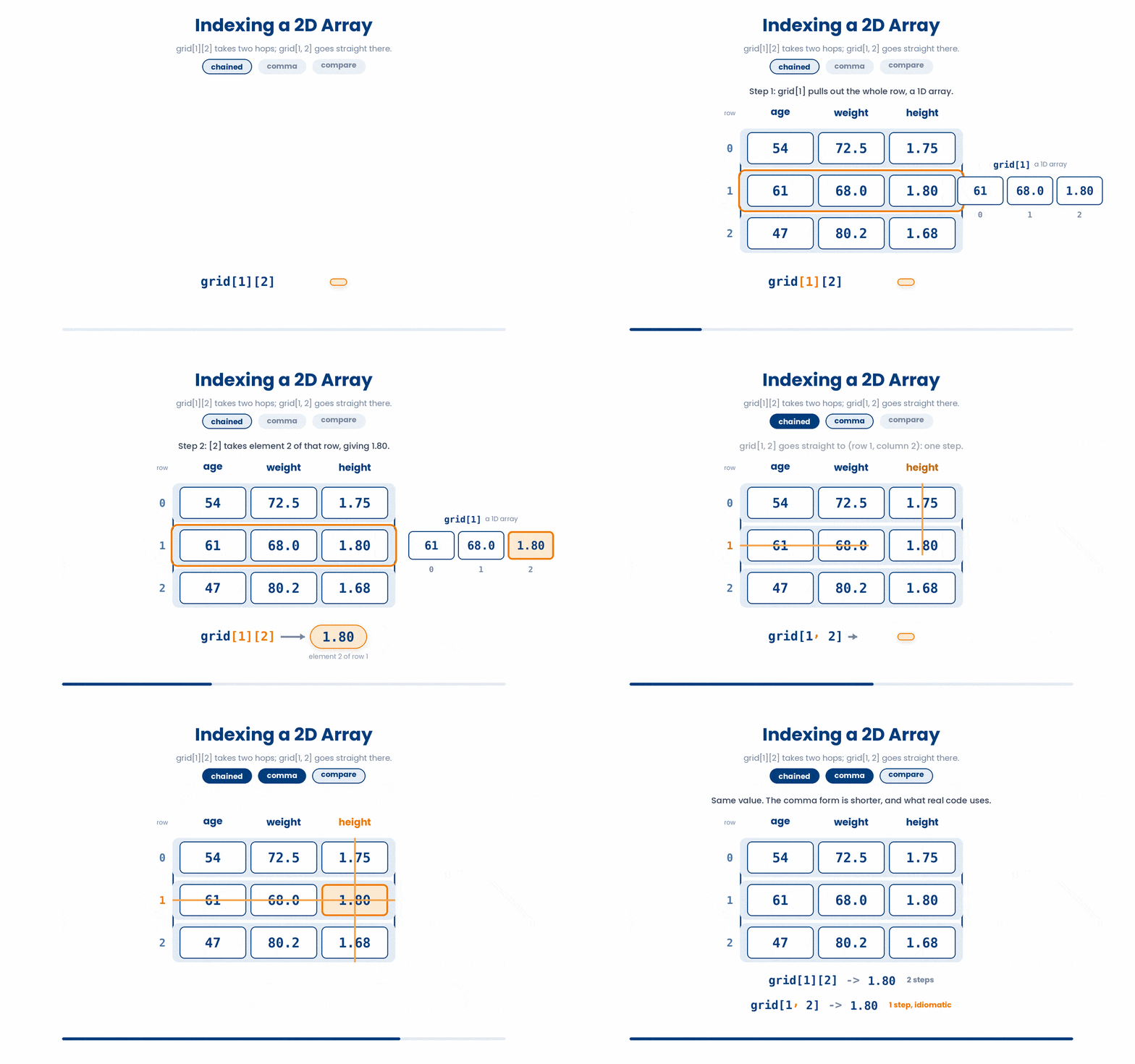
A common trip-up: with a list of lists in plain Python you would write grid[1][2] - two pairs of brackets, indexing one list out of the outer list and then one element out of that. With a NumPy array the comma form grid[1, 2] is the idiomatic way. grid[1][2] still works on most arrays, but the comma form is faster, more flexible (it gives you slices like [:, 0] for free), and what you will see in real code.
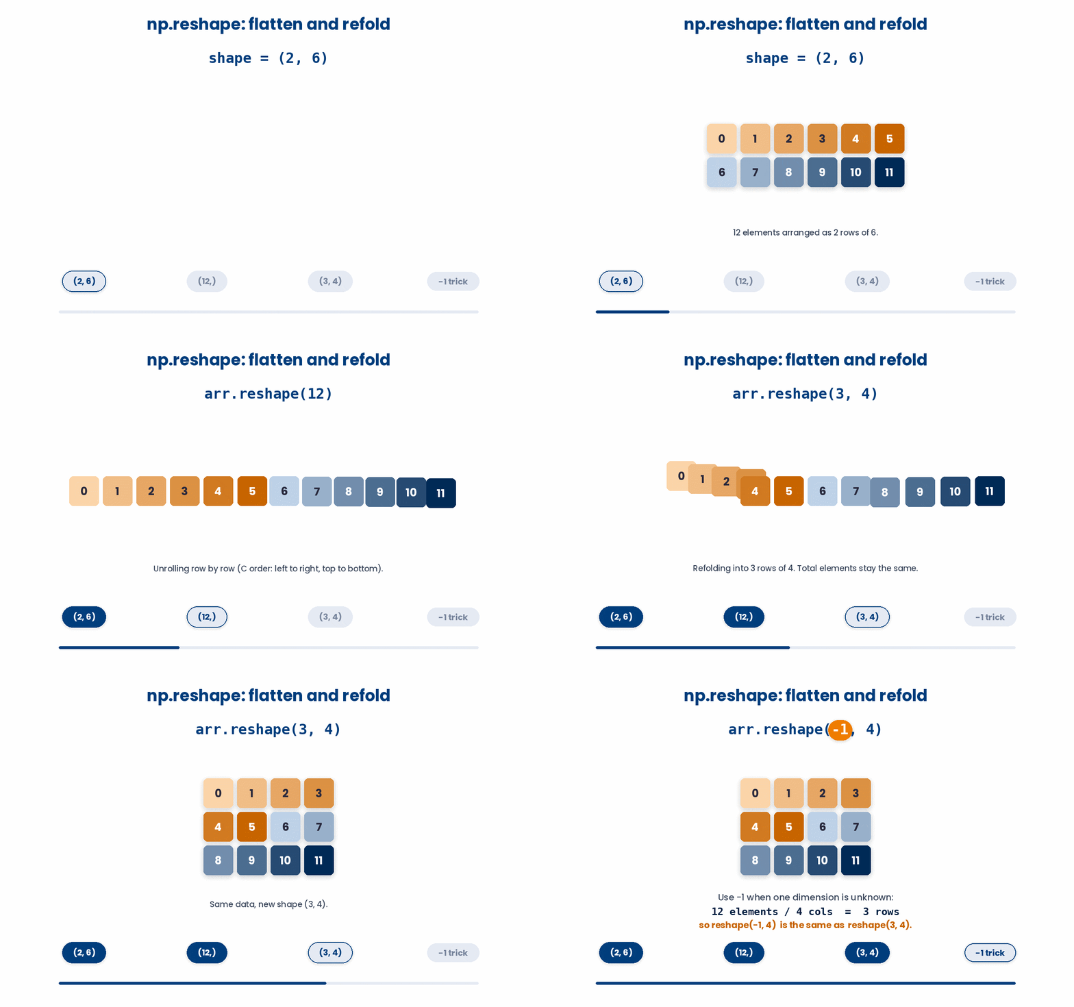
One more useful tool is reshape, which gives you a view of an array with the same data laid out in a different shape. Reshaping is handy when you have a long 1D array of numbers but really they should be thought of as a grid - say twelve readings that are three patients with four measurements each.
Read the code carefully and type what you think it will print. Click Submit prediction for AI tutor feedback comparing your prediction against the real output, then click Reveal actual output to run the snippet yourself and see what happens.
import numpy as np
x = np.arange(12)
y = x.reshape(3, 4)
print(y.shape)The product of the dimensions in the new shape has to equal the total number of elements - 3 * 4 = 12, which matches np.arange(12). If the numbers do not match, NumPy raises a ValueError telling you so.
reshape groups a flat array into more dimensions. .flatten() does the reverse: it collapses an array of any shape back down to one dimension, reading it out row by row. You need this before almost any operation that expects a single flat list of numbers - a histogram of every pixel in an image, for instance, first needs that 2D grid flattened into one long run of values.
Try this snippet in the Python Scratchpad on the right.
import numpy as np
grid = np.array([[1, 2, 3], [4, 5, 6]])
print(grid.flatten()).ravel() does the same collapse and is often faster, because it hands back a view onto the original data whenever it can, rather than a fresh copy - the same view/copy distinction you met with .reshape(). .flatten() always copies, which costs a little memory but guarantees that changing the flattened array can never change the array it came from.
7.1 The reshape(-1, 1) idiom
A 1D array of n values has shape (n,). Many downstream tools want a 2D column vector of shape (n, 1) instead - one column with n rows. The trick is .reshape(-1, 1). The -1 tells NumPy to work out that dimension itself given the total number of elements, so you do not have to count.
Try this snippet in the Python Scratchpad on the right.
import numpy as np
ages = np.array([54, 61, 47, 72, 38])
print(ages.shape)
column = ages.reshape(-1, 1)
print(column)
print(column.shape)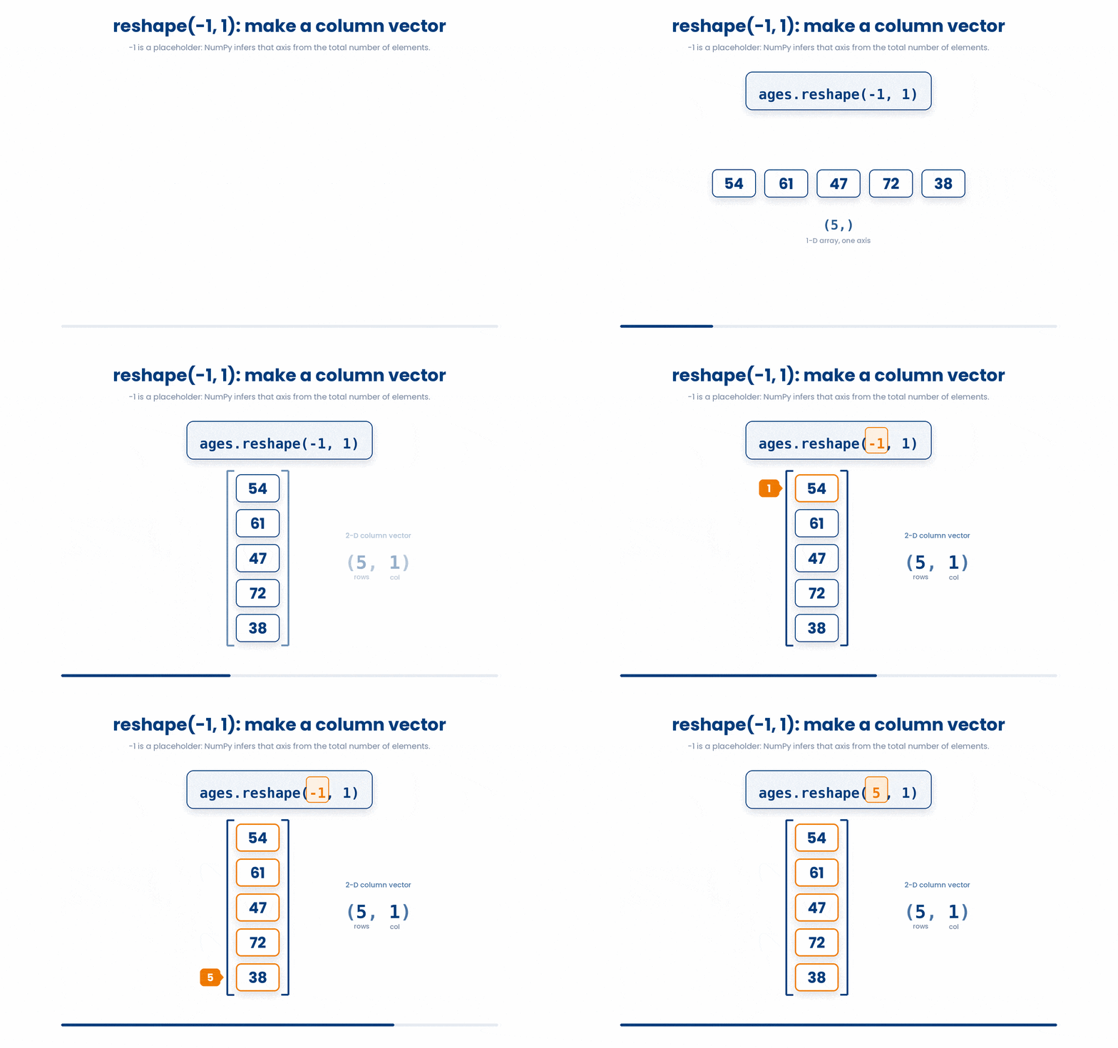
8 Check your understanding
You have reached the end of the module. Try the same questions again — your answers here, paired with your pre-test answers, are how we measure what the module taught you. Answer every question and confidence rating, then click Submit and see results to view your score.
What happens when you write arr.shape() with parentheses, on a NumPy array?
What is the dtype of np.array([54, 61, 72.5])?
What does np.arange(0, 10, 2) produce?
You have arr = np.array([1, 2, 3, 4]). What does arr * 2 produce?
What does np.sqrt(np.array([1, 4, 9, 16])) return?
For ages = np.array([54, 61, 47, 72, 38]), what does ages[1:4] return?
You have a 2D array m with shape (3, 4). What does m[:, 0] return?
For ages = np.array([54, 61, 47, 72, 38]), what shape does ages.reshape(-1, 1) give?
I can build a NumPy array from a Python list and read its shape, dtype, and size attributes.
I can do element-wise arithmetic on a NumPy array, index single values and slices of a 1D or 2D array, and reshape an array into a different shape.
9 Your results
Here is how your post-test answers compare with your pre-test answers. The pre/post pairing is the most reliable way to see what this module actually taught you.
Submit the post-test to see your results.
What is the one thing from this module that is still unclear to you?