

1 Introduction
A model is built from patients we already have. It is then used on patients we have not seen yet: the next person in clinic, or patients in another hospital. So the real test of a model is not how well it fits the patients it learned from. It is how well it predicts for new patients. A model that does this well is said to generalise.
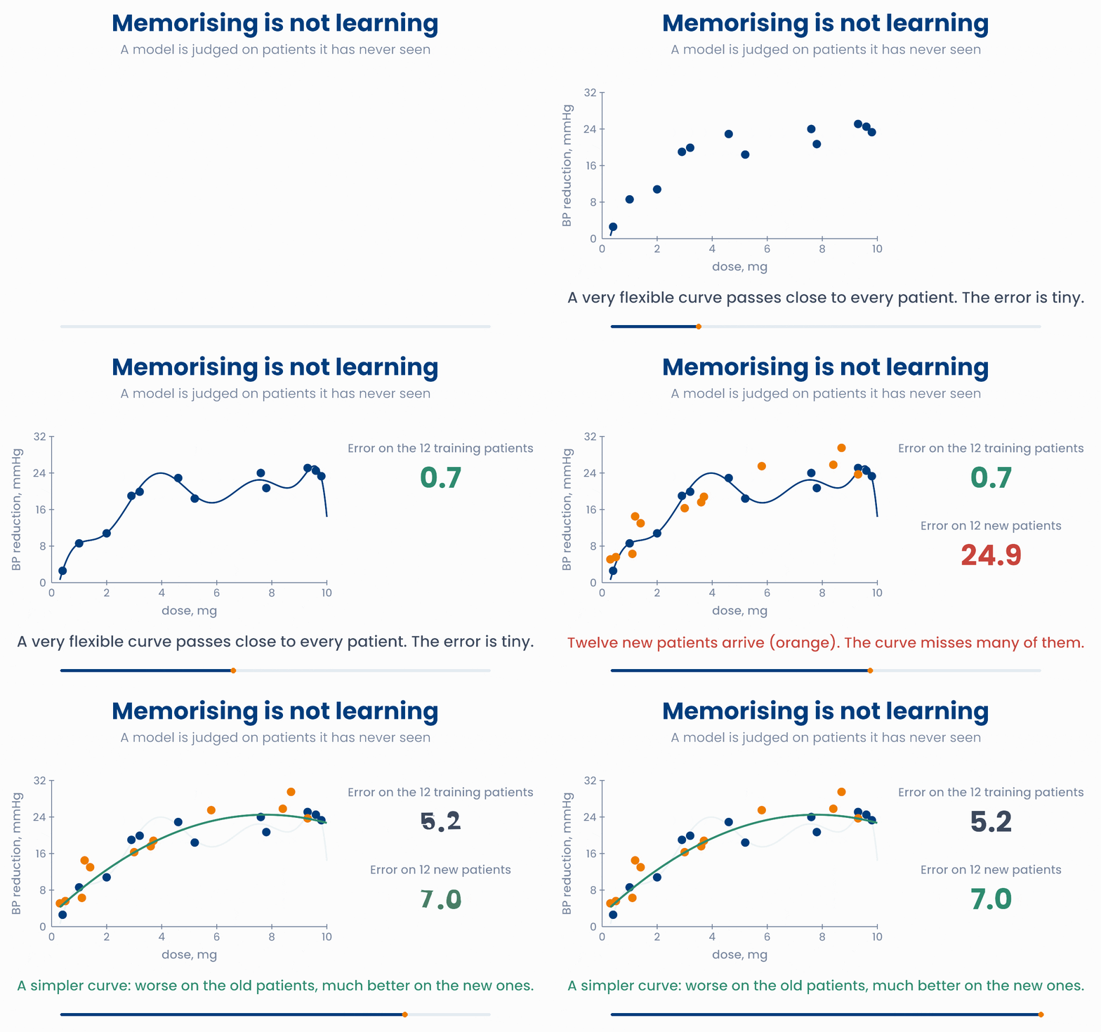
In the animation, twelve patients took different doses of a blood-pressure drug. A very flexible curve passes close to all twelve. Its error on them (the MSE from lesson 6.1, in mmHg²) is only 0.7. But on twelve new patients its error is 24.9. A simpler curve is a little worse on the first twelve (5.2) and much better on the new ones (7.0).
The flexible curve has memorised the twelve patients, including random ups and downs that will not happen again. A student who memorises the answers to last year's exam can still fail this year's exam. The same is true for models.
What you will be able to do
- Recognise underfitting and overfitting.
- Explain why we keep test patients aside, and read a plot of training and test error.
- Describe bias and variance, and how a penalty on the weights (ridge or lasso) controls overfitting.
2 Underfitting and overfitting
The twelve patients follow a typical dose–response pattern: the fall in blood pressure rises quickly at low doses and then levels off. Each patient also has some noise: random variation from the measurement, the time of day, and many things we do not record.
In lesson 1.2 you fitted curves with polynomials. The degree of the polynomial sets how flexible the model is. A degree-1 line cannot bend. A degree-9 polynomial can bend up to eight times.
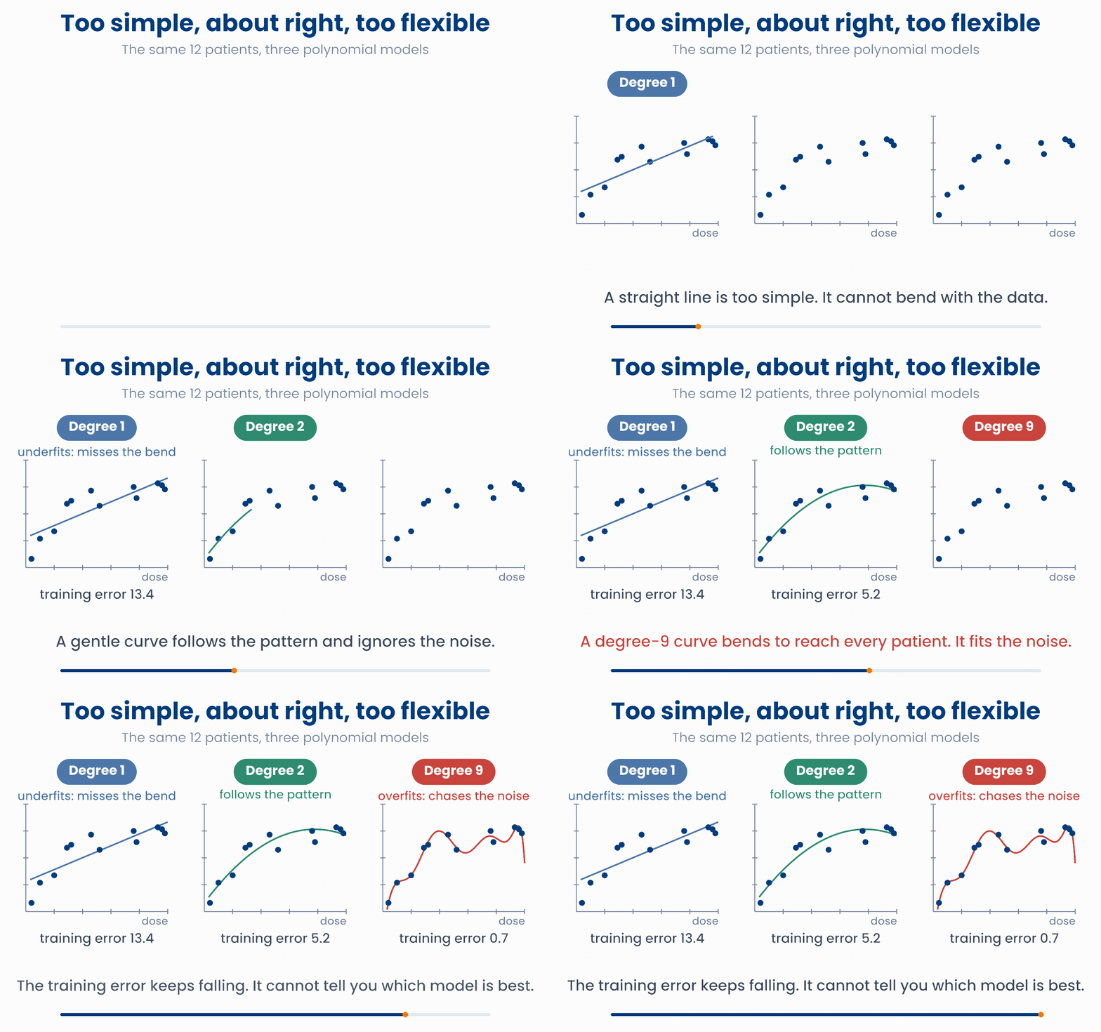
- Underfitting: the model is too simple to follow the real pattern. The straight line misses the bend, so it is wrong in the same way for many patients.
- Overfitting: the model is so flexible that it follows the noise as well as the pattern. The degree-9 curve wiggles to reach single patients. The wiggles are not real biology, so they will be wrong for the next patient.
- In between, the degree-2 curve follows the pattern and ignores most of the noise.
Move one patient and watch the curve
Choose a model. Then drag any patient up or down. The straight line hardly moves. The degree-9 curve bends to chase the patient you move: it is fitting the noise.
Look at the training error as you change the model: it is lowest for degree 9. A more flexible model always fits its training patients at least as well as a simpler one. So the training error cannot tell you when to stop. The next section shows what can.
import numpy as np
x = np.array([0.4, 1, 2, 2.9, 3.2, 4.6, 5.2, 7.6, 7.8, 9.3, 9.6, 9.8])   # dose, mg
y = np.array([2.6, 8.6, 10.8, 19, 19.9, 22.9, 18.4, 24, 20.7, 25.1, 24.5, 23.3])
u = x / 5 - 1                     # rescale 0..10 mg to -1..1 (keeps high powers tame)
for d in [1, 2, 9]:
    coef = np.polyfit(u, y, d)    # least squares polynomial of degree d
    print(d, round(np.mean((y - np.polyval(coef, u)) ** 2), 1))
# 1 13.4 / 2 5.2 / 9 0.7 training error falls as the degree risesA model predicts HbA1c from 15 blood tests. On the 300 patients it was trained on, its error is 0.01. On the next 300 patients it is 1.8. What is the most likely problem?
3 Training and test data
To see how a model does on new patients, keep some patients aside. Before fitting, split the data into two groups:
- The training set: the patients the model learns from.
- The test set: patients the model never sees while it learns. The error on them estimates how the model will do on new patients.
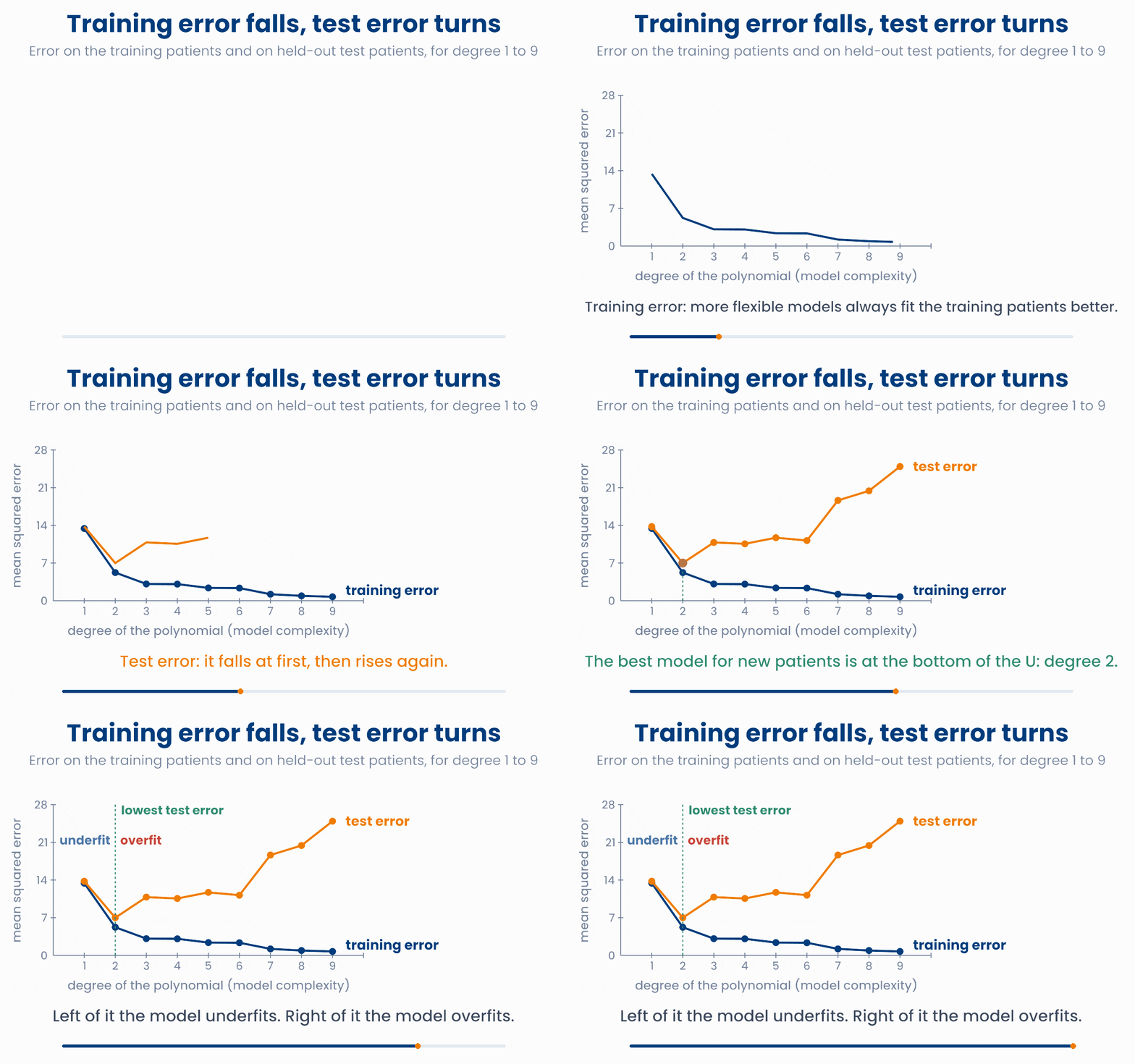
As the degree goes up, the training error keeps falling. The test error falls at first, then rises again: it makes a U shape. The bottom of the U, here degree 2, is the model that will do best on new patients.
Training error falls, test error turns
Move the degree. The top plot shows the curve with the training patients (blue) and the test patients (orange). The bottom plot shows both errors for every degree, with your choice marked.
Validation and cross-validation
Data leakage
import numpy as np
rng = np.random.default_rng(0)
dose = rng.uniform(0, 10, 24)                            # 24 made-up patients
fall = 30 * dose / (dose + 2) + rng.normal(0, 3, 24)
idx = rng.permutation(24); tr, te = idx[:12], idx[12:]   # hold out 12 patients
for d in [1, 2, 9]:
    c = np.polyfit(dose[tr] / 5 - 1, fall[tr], d)        # fit on the training patients only
    err = (fall - np.polyval(c, dose / 5 - 1)) ** 2
    print(d, round(err[tr].mean(), 1), round(err[te].mean(), 1))
# 1 22.6 26.0 / 2 5.4 9.9 / 9 0.3 352.0 training error, then test errorTwo models predict length of stay. Model A: training error 2.1, test error 2.3. Model B: training error 0.4, test error 6.5. Which model should the hospital use for new patients?
4 Bias and variance
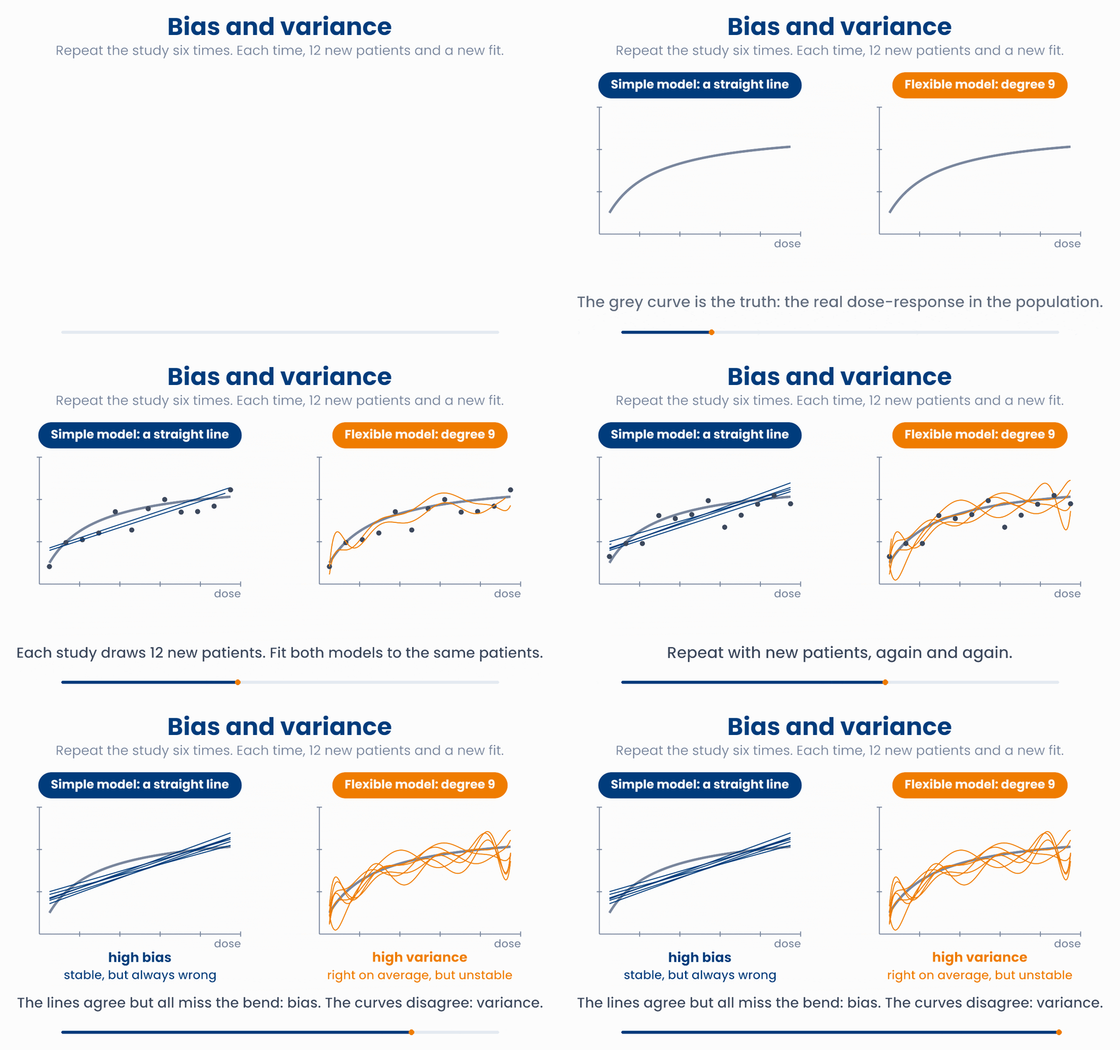
Imagine running the same study many times. Each time you recruit new patients from the same population and fit the same kind of model. Two different things can go wrong:
- Bias: the model is wrong in the same way every time. A straight line always misses the bend at low doses. More patients do not fix this.
- Variance: the model changes a lot when the training patients change. A degree-9 curve is right on average, but every study gives a very different curve.
Repeat the study: bias and variance
Press New study, or Run 20 studies. Each study draws new patients and fits both models. Compare how the two models change from study to study. Then try 192 patients per study.
Simple models have high bias and low variance. Flexible models have low bias and high variance. The error on new patients contains both, plus noise that no model can predict:
This is the bias–variance trade-off. On the left of the U-curve, bias is the problem: the model underfits. On the right, variance is the problem: the model overfits. The best model balances the two.
More data reduces variance
import numpy as np
rng = np.random.default_rng(2)
dose = np.linspace(0.5, 9.5, 12)
for d in [1, 9]:
    pred = []
    for study in range(1000):                    # repeat the study 1,000 times
        fall = 30 * dose / (dose + 2) + rng.normal(0, 3, 12)
        c = np.polyfit(dose / 5 - 1, fall, d)
        pred.append(np.polyval(c, 1 / 5 - 1))    # prediction at 1 mg
    print(d, round(np.mean(pred) - 10, 1), round(np.std(pred), 1))
# 1 2.4 1.5   line: about 2.4 too high every time (bias), but stable
# 9 0.1 6.2 degree 9: right on average (truth 10), but spread widelyA hospital retrains a risk model every month on that month's patients. Each month the model gives very different predictions for the same kind of patient. What does the model have, and what would help?
5 Regularisation: a penalty for large weights
Choosing a lower degree is one way to stop overfitting. Another way keeps the flexible model, but makes large weights costly. Overfit models usually have huge weights. The degree-9 fit in this lesson has a weight of more than 1,000: large positive and negative terms almost cancel, and what is left over makes the wiggles. Regularisation adds a penalty for large weights to the loss:
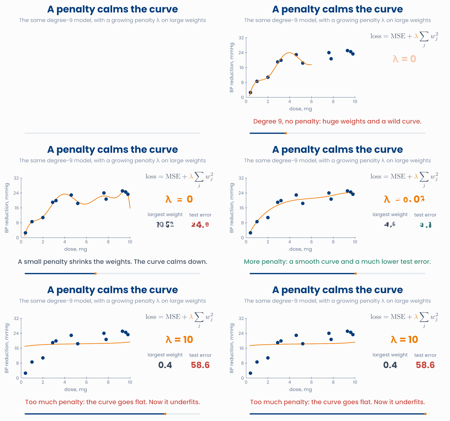
Now the optimiser has two goals: fit the patients (a small MSE) and keep the weights small (a small penalty). λ sets the balance:
- \(\lambda = 0\): no penalty. The degree-9 model overfits. Test error 24.9.
- A moderate \(\lambda\) (0.03 here): the curve is smooth. Test error 9.1.
- A very large \(\lambda\) (10): every weight is pushed almost to 0. The curve goes flat, and the model underfits. Test error 58.6.
There are two common ways to measure the "size of the weights":
| Name | Penalty | What it does |
|---|---|---|
| L2, or ridge | \(\lambda \sum_j w_j^2\) | Shrinks all the weights smoothly towards 0. None of them becomes exactly 0. |
| L1, or lasso | \(\lambda \sum_j |w_j|\) | Shrinks the weights, and sets some of them exactly to 0. The model then ignores those inputs. |
Ridge and lasso on the degree-9 model
Move λ from 0 upwards and watch the curve calm down and the weights shrink (the bars use a log scale). Then switch to lasso: weights drop to exactly 0 one by one. Push λ to the end: the curve goes flat.
Why lasso matters in precision health. A gene-expression study may measure 20,000 genes in 200 patients. A linear model with one weight for each gene has far more weights than patients. Least squares then has no single answer: there are endless ways to fit the 200 patients perfectly, and all of them overfit. Lasso keeps a small set of genes and sets the weights of all the others to exactly zero. The result is a short list of genes that can be checked in the laboratory: a gene signature.
Why you will care later
import numpy as np
x = np.array([0.4, 1, 2, 2.9, 3.2, 4.6, 5.2, 7.6, 7.8, 9.3, 9.6, 9.8])   # dose, mg
y = np.array([2.6, 8.6, 10.8, 19, 19.9, 22.9, 18.4, 24, 20.7, 25.1, 24.5, 23.3])
X = np.vander(x / 5 - 1, 10, increasing=True)[:, 1:]   # powers 1 to 9
Xc, yc = X - X.mean(0), y - y.mean()       # centre: the intercept is not penalised
n, p = X.shape
for lam in [0, 0.0001, 0.03, 10]:          # ridge: minimise MSE + lam * sum(w**2)
    w = np.linalg.solve(Xc.T @ Xc / n + lam * np.eye(p), Xc.T @ yc / n)
    print(lam, round(np.abs(w).max(), 1))  # the largest weight
# 0 1052.0 / 0.0001 37.2 / 0.03 4.9 / 10 0.4You fit a lasso model to the expression of 5,000 genes. What happens as you make λ larger?
6 Where you go from here
This is the end of the course. You now have the mathematics that statistics and machine learning are built on. Here is a map from each unit to where you will meet it again.
| Unit | You learned | Where it comes back |
|---|---|---|
| 1 Functions and notation | \(\Sigma\) and \(\Pi\), lines, exponentials, logs, odds, the sigmoid | Reading any formula in a paper; log fold changes in genomics; odds ratios; logistic regression |
| 2 Linear algebra | Vectors, matrices, \(\hat{y} = X\beta\) | Multiple regression; principal component analysis (PCA); every layer of a neural network |
| 3 Calculus | Derivatives, partial derivatives, gradients, areas under curves | Training any model by gradient descent; drug concentration over time; probabilities as areas |
| 4 Probability | Conditional probability, Bayes' theorem, distributions | Diagnostic tests and screening; Bayesian statistics; simulation |
| 5 Statistical foundations | Samples, standard error, correlation, likelihood, least squares | Confidence intervals and p-values; fitting linear, logistic and survival models |
| 6 Optimisation | Loss functions, gradient descent, overfitting, regularisation | Machine learning: cross-validation, lasso gene signatures, neural networks |
Methods you are now ready to learn:
- Linear regression
- Logistic regression
- Survival analysis and Cox models
- Principal component analysis
- Clustering
- Ridge, lasso and elastic net
- Cross-validation
- Decision trees and random forests
- Neural networks
- Polygenic risk scores
- Bayesian statistics
Four questions for any model you meet
- What is the model? Which inputs does it use, and what are its weights?
- What is the loss? MSE, log loss, or something else?
- How are the weights found? A direct formula, or gradient descent?
- How was it tested? On patients it had never seen, and without leakage?
You do not need to remember every formula from this course. When you meet one, read it from the inside out, as in lesson 1.1, and ask these four questions. That is what working statisticians and machine-learning scientists do every day. Well done for reaching the end.
7 Check your understanding
Five short questions on this lesson. Nothing is graded or saved outside this browser. If you choose a wrong option you get a hint, and you can try again.
A straight-line model has a training error of 25 and a test error of 26. A curve that can bend has errors of 6 and 7. What was wrong with the straight line?
A study has 3 skin images from each of 500 patients. The images are shuffled and split at random into a training set and a test set. What is the problem?
The test errors for polynomial degrees 1 to 6 are 14, 7, 9, 11, 12 and 16. Which degree would you choose for new patients?
Which sentence describes high variance?
A ridge model is fitted with a very large λ. What do you expect?