

1 Introduction
A clinic tests a new blood-pressure drug on five patients. Each patient gets a different dose, and the clinic records how much their systolic blood pressure falls. The question is: how many mmHg does each extra mg of the drug lower the pressure?
A computer can answer this by "learning" from the five patients. In machine learning, learning means something plain: change the numbers inside a model until its errors are as small as possible.
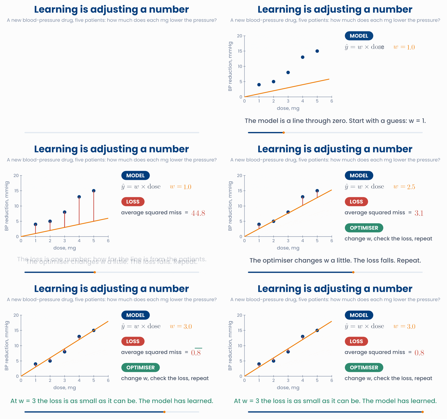
Every learning method has the same three parts:
| Part | In the animation | In general |
|---|---|---|
| Model | \(\hat{y} = w \times \text{dose}\) | A formula with numbers that can be changed, called weights. |
| Loss | the average squared miss | One number that says how wrong the model is on the patients. |
| Optimiser | change \(w\), check the loss, repeat | A rule that changes the weights to make the loss smaller. |
The number \(w\) is a weight. Statisticians call it a parameter or coefficient and often write it as \(\beta\). The model in the animation has one weight. Linear regression has one weight for each measurement, as in \(\hat{y} = X\beta\) from Unit 2. A neural network that reads chest X-rays has millions of weights. The idea is the same for all of them.
What you will be able to do
- Say what a loss function measures, and choose mean squared error or log loss for a problem.
- Describe gradient descent in words: measure the slope, step downhill, repeat.
- Explain what the learning rate does, and spot a learning rate that is too large.
import numpy as np
dose = np.array([1, 2, 3, 4, 5])        # mg
drop = np.array([4, 5, 8, 13, 15])      # fall in systolic BP, mmHg
for w in [1, 2, 3, 4]:
    loss = np.mean((drop - w * dose) ** 2)   # average squared miss
print(w, round(loss, 1)) # 1 44.8 / 2 11.8 / 3 0.8 / 4 11.82 Loss: one number for how wrong
For each patient \(i\), the model makes a prediction \(\hat{y}_i\), and we know the true value \(y_i\). The difference \(y_i - \hat{y}_i\) is the residual, or miss, from Unit 5. A hospital model may learn from 50,000 patients, so it has 50,000 misses. To improve the model, the computer needs to turn them all into one number. That number is the loss (also called the cost).
- A loss of 0 means every prediction is exactly right.
- Lower is better. Training a model means making its loss as small as possible.
The first idea most people have is to average the misses. This does not work. A patient who stays 3 days longer than predicted gives +3. A patient who stays 3 days less gives −3. Together they cancel to 0. A very poor model can have an average miss of zero.
Why the misses cannot simply be added
Each dot is a patient. The line predicts length of stay from a frailty score. Change its slope. The plain misses always cancel to zero. The absolute and the squared misses do not, and they are smallest when the line fits well.
So a loss first turns each miss into a penalty that is never negative. Then it takes the average over all \(n\) patients. This is the sigma from lesson 1.1:
Which penalty to use depends on what the model predicts:
| The model predicts | Examples | Usual loss |
|---|---|---|
| A number | HbA1c, length of stay, a drug level | Mean squared error (next section) |
| The probability of "yes" | readmission within 30 days, malignant or benign | Log loss, also called cross-entropy (section 4) |
Why you will care later
import numpy as np
frailty = np.array([1, 2, 3, 4, 5, 6, 7, 8])
stay = np.array([2, 4, 3, 6, 5, 8, 8, 12])     # length of stay, days
pred = 6 + 1.2 * (frailty - 4.5)               # a line through the centre
miss = stay - pred
print(round(miss.mean(), 2))            # 0.0   the + and - misses cancel
print(round(np.abs(miss).mean(), 2))    # 0.95  mean absolute error, days
print(round((miss ** 2).mean(), 2)) # 1.21 mean squared error, days²A model predicts the length of stay of four patients. Its misses are +3, −3, +1 and −1 days. What is the average miss, and what does it tell you?
3 Mean squared error
When a model predicts a number, such as HbA1c, blood pressure or length of stay, the usual loss is the mean squared error (MSE). Square each miss, then take the mean:
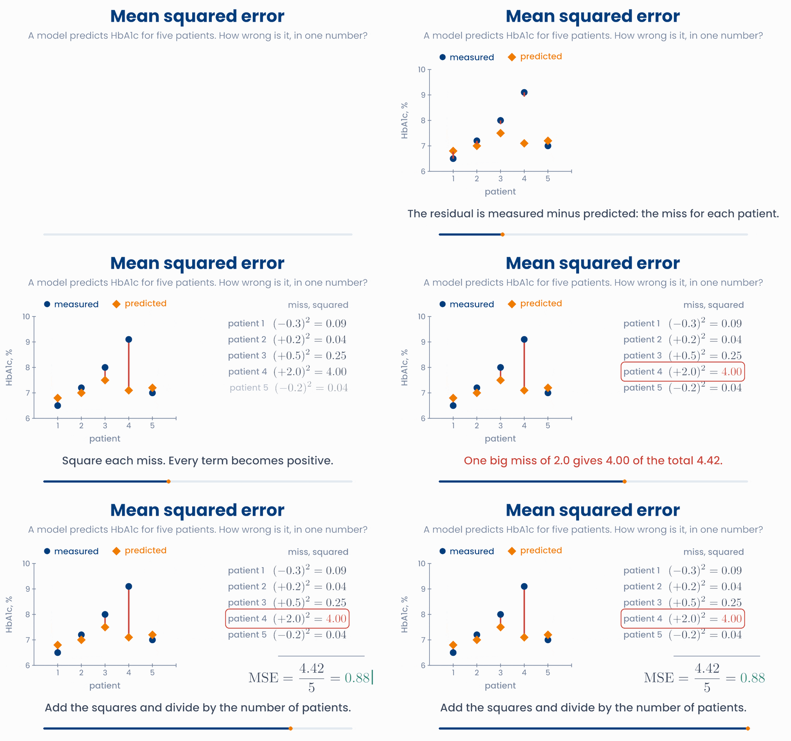
Squaring does two jobs:
- Every penalty is positive, so misses cannot cancel.
- Big misses count much more than small ones. A miss of 0.5 counts 0.25. A miss of 2.0 counts 4.00: it is 4 times as big, but it counts 16 times as much. A model trained with the MSE tries very hard to avoid big misses.
The MSE is the average area of the squares
Drag on the left or the right half of the plot to move that end of the line. Each square has a side equal to one patient's miss, so its area is the squared miss. Make the squares small. Then add the unusual patient and watch one square take over.
Watch the units. HbA1c is measured in %, so its MSE is in "% squared", which is hard to imagine. The square root brings it back to the units of the data. This is the root mean squared error (RMSE). It is the typical size of a miss:
In the animation \(\text{MSE} = 0.884\), so \(\text{RMSE} = \sqrt{0.884} \approx 0.94\). The predictions are typically about 0.9 percentage points away from the measured HbA1c.
You have met this before
import numpy as np
measured = np.array([6.5, 7.2, 8.0, 9.1, 7.0])     # HbA1c, %
predicted = np.array([6.8, 7.0, 7.5, 7.1, 7.2])
miss = measured - predicted
print(np.round(miss ** 2, 2))      # [0.09 0.04 0.25 4.   0.04]
mse = np.mean(miss ** 2)
print(round(mse, 3))               # 0.884  in %²
print(round(np.sqrt(mse), 2)) # 0.94 the RMSE, back in %Two models predict the length of stay of the same four patients. Model A misses every patient by 1 day. Model B is exactly right for three patients and misses the fourth by 4 days. Which model has the larger MSE?
4 Log loss for probabilities
Many clinical models do not predict a number. They predict the probability of a yes/no outcome. Will this patient be readmitted within 30 days? Is this tumour malignant? In lesson 1.2 you saw how the sigmoid turns a risk score into a probability \(p\) between 0 and 1. The true outcome is \(y = 1\) (yes) or \(y = 0\) (no).
The loss for such a model asks one question: what probability did the model give to what really happened? A good model gives a high probability to the truth. The penalty is minus the log of that probability:
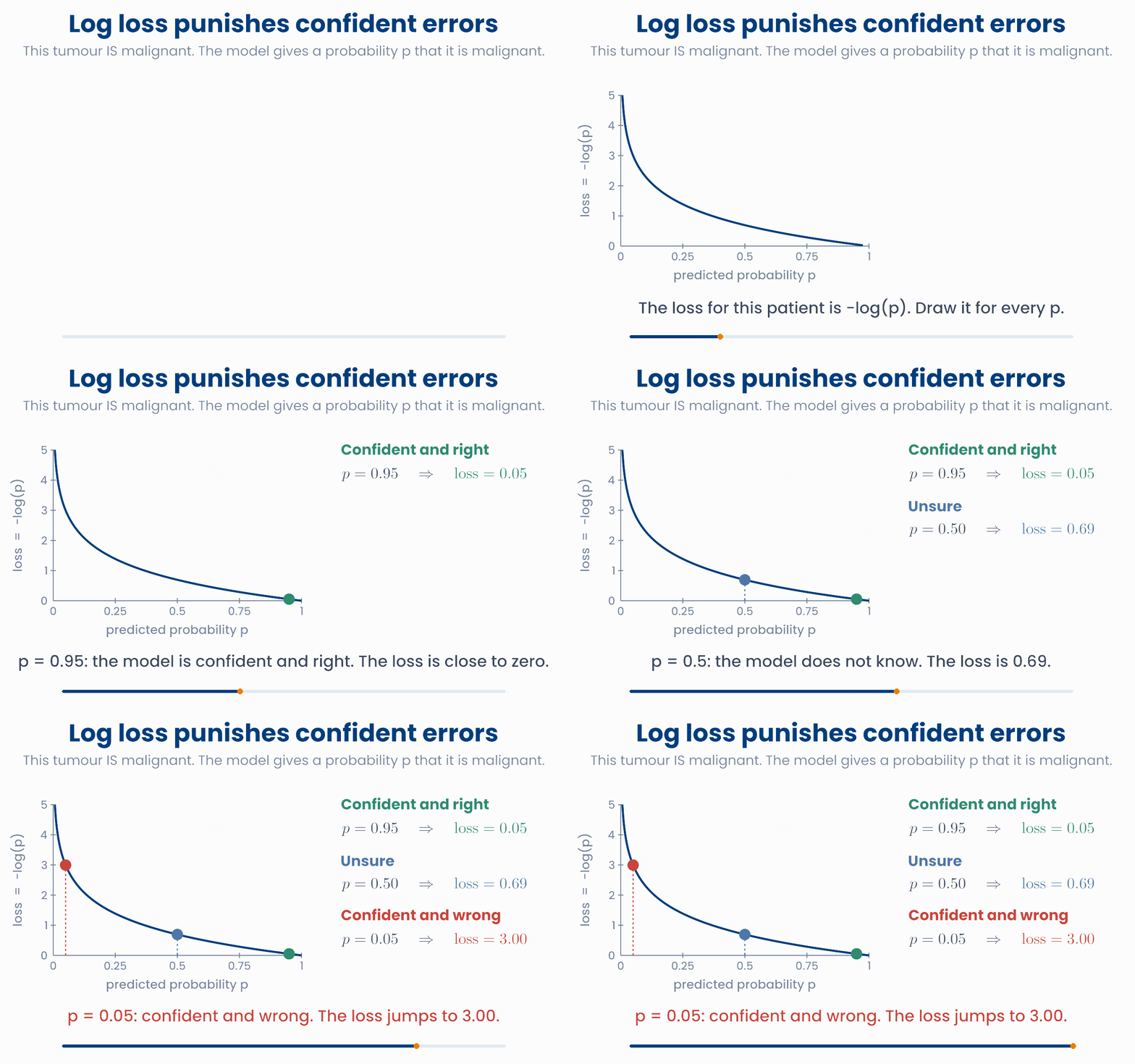
- Confident and right (\(p = 0.95\) for a malignant tumour): the loss is \(-\log 0.95 = 0.05\). Almost no penalty.
- Unsure (\(p = 0.5\)): the loss is \(-\log 0.5 = 0.69\).
- Confident and wrong (\(p = 0.05\)): the loss is \(-\log 0.05 = 3.00\). As \(p\) goes towards 0, the loss grows without limit.
Confident and wrong is punished hardest
Choose what the tumour really is. Then move the model's probability that it is malignant. Tick the box to compare with the squared error, which can never be more than 1.
Written as one formula for \(n\) patients, with each \(y_i\) equal to 1 or 0, this is the log loss, also called binary cross-entropy:
Why you will care later
import numpy as np
y = np.array([1, 0, 1, 0])               # 1 = malignant, 0 = benign
p = np.array([0.9, 0.2, 0.6, 0.05])      # model's probability of malignant
penalty = -(y * np.log(p) + (1 - y) * np.log(1 - p))
print(np.round(penalty, 3))              # [0.105 0.223 0.511 0.051]
print(round(penalty.mean(), 3)) # 0.223 the log lossA tumour is benign (\(y = 0\)). A model gives a probability \(p\) that it is malignant. Which value of \(p\) gives the largest log loss?
5 Gradient descent: walk downhill
We now have a loss. How does the computer find the weights that make it smallest?
Go back to the drug in the introduction. For every possible weight \(w\) we can work out the loss. Drawn as a curve, this is the loss landscape, and we want its lowest point. With one weight you could try every value. But a real model may have a million weights, and trying every combination is impossible.
Instead, the computer does what a walker on a hillside in thick fog would do: feel which way the ground slopes, and take a step downhill. Unit 3 gave you the tool for this. The derivative is the slope of a curve, and at the lowest point the slope is zero.
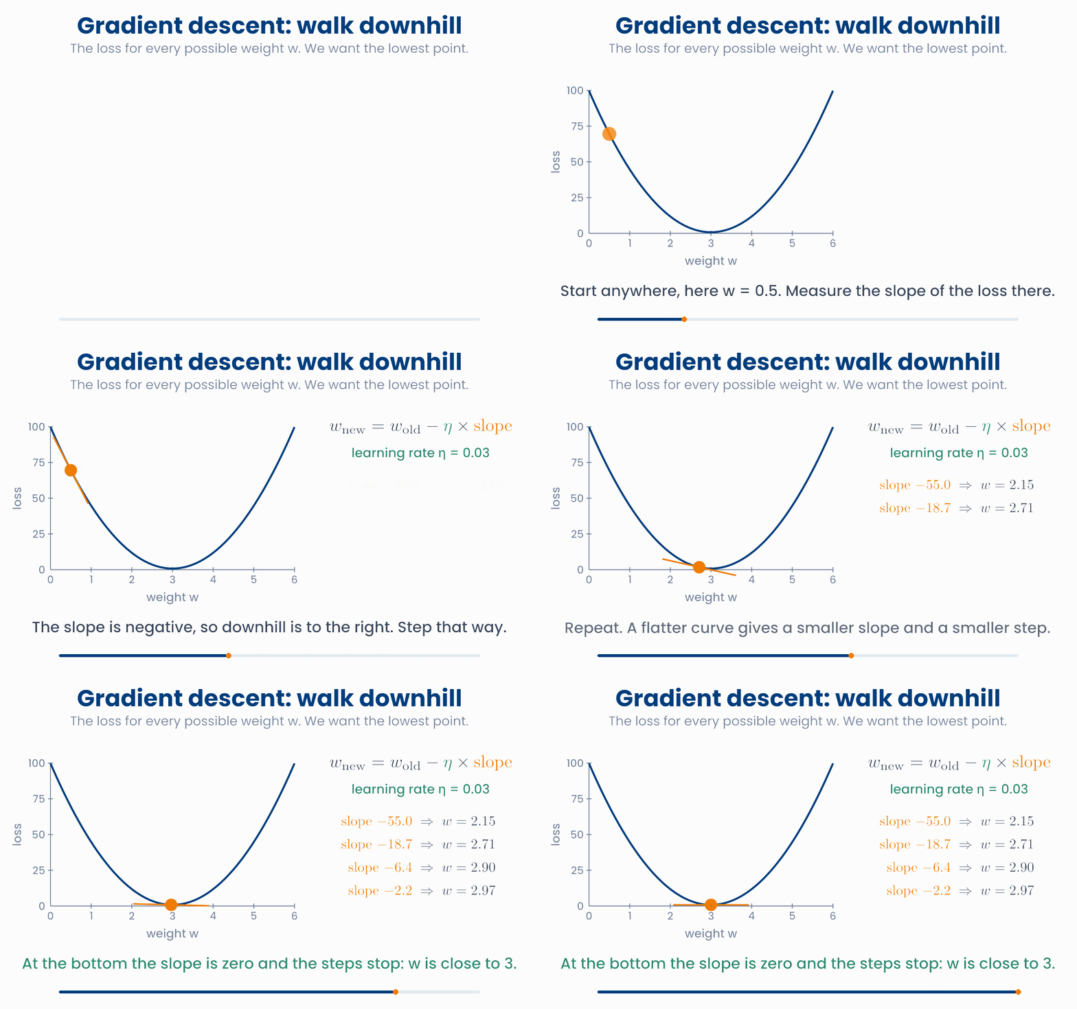
This method is called gradient descent. The rule for one step is:
- If the slope is negative, the loss goes down to the right. The minus sign makes \(w\) bigger: the step goes to the right.
- If the slope is positive, the step goes to the left.
- A steep slope gives a big step. Near the bottom the slope is small, so the steps are small. At the bottom the slope is 0, and \(w\) stops changing.
The first steps in the animation
- Start at \(w = 0.5\). For this loss, the slope at any \(w\) is \(22 \times (w - 3)\). (The computer works this out with the rules of Unit 3.) Here it is \(22 \times (-2.5) = -55\).
- Step: \(w = 0.5 - 0.03 \times (-55) = 0.5 + 1.65 = 2.15\).
- New slope: \(22 \times (2.15 - 3) = -18.7\). Step: \(w = 2.15 + 0.03 \times 18.7 = 2.71\).
- Repeat. After two more steps \(w = 2.97\), very close to the bottom at 3.
Two weights. Now let the line have an intercept as well: \(\hat{y} = b + w \times \text{dose}\). The loss now depends on two numbers, so the landscape is a surface shaped like a bowl. We draw it from above, like a map, with contour lines that join points of equal loss. The gradient from Unit 3 is the list of the two slopes (the partial derivatives). It points uphill, so each step goes the opposite way:
Gradient descent on a map of the loss
Each point on the map is one line (an intercept b and a slope w). Click anywhere on the map to start there. The orange path shows every step downhill. The lower plot shows the line for the current point.
The path does not head straight for the centre. This loss is a long, narrow valley. The first steps drop quickly to the floor of the valley. Then many small steps walk along it to the bottom, at \(b = 0\) and \(w = 3\). The best line goes through zero, as in the introduction.
import numpy as np
dose = np.array([1, 2, 3, 4, 5])
drop = np.array([4, 5, 8, 13, 15])
w, lr = 0.5, 0.03                                   # starting guess and learning rate
for step in range(20):
    slope = np.mean(-2 * dose * (drop - w * dose))  # slope of the MSE at this w
    w = w - lr * slope                              # one step downhill
print(round(w, 3))                                  # 3.0
print(round(np.mean((drop - w * dose) ** 2), 3)) # 0.8 the lowest lossAt the current weight, the slope of the loss is +8 and the learning rate is 0.1. What does one step of gradient descent do?
6 The learning rate
The learning rate \(\eta\) sets the size of each step. It is not learned from the data: you choose it before training starts. A setting like this is called a hyperparameter.
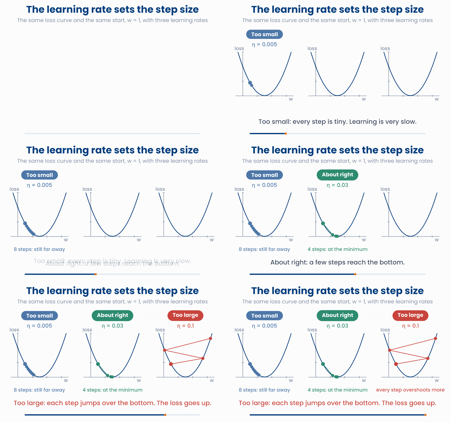
- Too small (\(\eta = 0.005\)): every step is tiny. After 8 steps the weight is still far from the bottom. Training is slow.
- About right (\(\eta = 0.03\)): a few steps reach the bottom.
- Too large (\(\eta = 0.1\)): each step jumps over the bottom and lands higher up on the other side. The loss grows with every step. This is called divergence.
Find a learning rate that works
Choose a learning rate, then press Step or Run. The lower plot shows the loss after each step. Try 0.005, 0.03, 0.06, 0.09 and 0.1.
The lower plot in the figure is a loss curve (or learning curve): the loss after each step. People who train models look at it all the time. A healthy loss curve falls fast at first, then flattens. A loss curve that jumps about or climbs means that the learning rate is too large.
Two things you will hear about
- Stochastic and mini-batch gradient descent. With a million patients, working out the slope over everyone for every step is slow. So each step uses a small random batch of patients, for example 32. The steps are noisier, but much cheaper.
- Local minima. Some loss landscapes have more than one valley. Gradient descent finds the bottom of the valley it starts in, which may not be the lowest one. The losses of linear and logistic regression are a single bowl, so this cannot happen there. For neural networks it can.
import numpy as np
dose = np.array([1, 2, 3, 4, 5])
drop = np.array([4, 5, 8, 13, 15])
for lr in [0.005, 0.03, 0.1]:
    w = 1.0
    for step in range(8):
        w = w - lr * np.mean(-2 * dose * (drop - w * dose))
    print(lr, round(w, 2))
# 0.005 2.21   too small: still on the way
# 0.03 3.0     about right: at the bottom
# 0.1 -5.6 too large: further away after every stepWhile a model trains, its loss after each step is 0.69, 0.72, 0.85, 1.40, 3.10. What is the most likely problem, and what should you do?
7 Putting it together
Now combine the three parts to fit a real kind of model. In lesson 1.2 you moved two sliders to fit an S-shaped curve to patients with and without diabetes. Here gradient descent does that job:
- Model: \(p = \sigma(\beta_0 + \beta_1 \times \text{glucose})\), the sigmoid of a straight line. This is logistic regression.
- Loss: the log loss over all 60 patients.
- Optimiser: gradient descent on \(\beta_0\) and \(\beta_1\), with learning rate 0.15, starting from \(\beta_0 = \beta_1 = 0\).
Watch a logistic regression learn
Press Run. The S-curve moves to fit the patients while the log loss falls in the lower plot. The computer takes 5,000 steps per second. Press Reset to start again.
Look at the two plots together:
- At the start \(\beta_0 = \beta_1 = 0\), so every patient gets \(p = 0.5\). The log loss is \(-\log 0.5 = 0.69\).
- The loss falls fast at first, then more and more slowly. Meanwhile the curve gets steeper and moves to the right.
- After 20,000 steps, \(\beta_0 \approx -8.71\), \(\beta_1 \approx 1.52\) and the loss has flattened at about 0.37. The data were made up with \(\beta_0 = -9\) and \(\beta_1 = 1.5\), so gradient descent has found values close to the truth. They are not exactly equal, because 60 patients are only a sample (Unit 5).
Twenty thousand steps may sound like a lot. Each step is cheap, and real models often take millions. The same three parts appear in every model you will meet:
| Method | Model | Loss | How the weights are found |
|---|---|---|---|
| Linear regression | \(\hat{y} = X\beta\) | MSE | A direct formula (least squares, Unit 5), or gradient descent |
| Logistic regression | \(p = \sigma(X\beta)\) | Log loss | Gradient descent, or a faster relative of it |
| Neural network | many layers of \(X\beta\), each passed through a simple function | MSE or log loss | Mini-batch gradient descent. The slopes come from the chain rule (Unit 3), in a method called backpropagation. |
Why you will care later
model.fit(X, y) in scikit-learn, or train a network in PyTorch, this loop is what runs: predict, measure the loss, work out the gradient, take a step. Knowing it helps you read a training log and fix common problems, such as a learning rate that is too large.import numpy as np
glucose = np.array([4.8, 5.5, 6.0, 6.6, 7.1, 7.9, 8.4, 9.2]) # mmol/L
disease = np.array([0, 0, 1, 0, 0, 1, 1, 1]) # 1 = diabetes
b0, b1, lr = 0.0, 0.0, 0.15
for step in range(20000):
p = 1 / (1 + np.exp(-(b0 + b1 * glucose))) # the model: sigmoid of a line
b0 = b0 - lr * np.mean(p - disease) # the two slopes of the log loss
b1 = b1 - lr * np.mean((p - disease) * glucose)
loss = -np.mean(disease * np.log(p) + (1 - disease) * np.log(1 - p))
print(round(b0, 1), round(b1, 2), round(loss, 2)) # -9.9 1.43 0.43During training, the log loss falls from 0.69 to 0.37 and then stays flat, step after step. What does the flat part tell you?
8 Check your understanding
Five short questions on this lesson. Nothing is graded or saved outside this browser. If you choose a wrong option you get a hint, and you can try again.
In machine learning, what does "training a model" mean?
A model predicts the systolic blood pressure of three patients. Its misses are +1, −2 and +3 mmHg. What is the mean squared error?
A patient was readmitted within 30 days (\(y = 1\)). Model A had given a probability of readmission of 0.6. Model B had given 0.1. Which model has the larger log loss for this patient?
A weight is \(w = 2\). The slope of the loss there is \(-4\), and the learning rate is 0.25. What is \(w\) after one step of gradient descent?
What happens if the learning rate is much too small?