

1 Introduction
A pharmacology team gives a new drug to 11 patients and measures how fast each patient's body clears it from the blood. Heavier patients tend to clear it faster. A simple model for this is:
The number \(\beta\) is a parameter: a number inside the model that we are free to choose. Each value of \(\beta\) gives a different line, and so different predictions. Fitting the model means choosing the value of \(\beta\) that agrees best with the data.
A model is a formula with a knob
Turn the knob β. The line is the model's prediction for each body weight. Find a value where the line runs through the middle of the patients.
By eye, several values of \(\beta\) close to 0.09 look reasonable. To let a computer choose one value, we need an exact rule for "agrees best". Statistics has two such rules, and this lesson covers both:
- Most likely. Choose the parameter value that makes the data we actually saw as probable as possible. This is maximum likelihood.
- Least error. Choose the parameter value that makes the model's errors as small as possible. This is least squares.
At the end of the lesson you will see that, for the most common models, the two rules give exactly the same answer.
Parameters are everywhere: the response rate \(p\) of a drug, the mean \(\mu\) of a lab value, the intercept and slope of a line. In Unit 2 you wrote a model as \(\hat{y} = X\beta\): the numbers in \(\beta\) are its parameters. A neural network has millions of parameters. The idea of fitting is the same for all of them.
What you will be able to do
- Say what a likelihood is, and read \(L(p)\) as a function of the parameter.
- Find the maximum likelihood estimate as the peak of a curve, and explain why we work with the log-likelihood.
- Work out residuals and the sum of squared residuals for a line.
- Explain why "most likely" and "smallest squared error" give the same line, and why "fitting means minimising a loss" is the idea behind regression and machine learning.
import numpy as np
weight = np.array([48, 54, 59, 63, 68, 72, 77, 83, 89, 96, 104])
clearance = np.array([3.9, 4.8, 6.3, 6.1, 5.1, 6.5, 6.6, 7.6, 7.0, 8.8, 9.5])

beta = 0.09                          # one choice of the parameter
predicted = beta * weight            # the model's clearance for every patient
print(predicted[:3])                 # [4.32 4.86 5.31]
print((clearance > predicted).sum()) # 6 patients above the line2 Likelihood
Start with the simplest model of all. A new drug is given to 20 patients, and 7 of them respond. The model says: each patient responds with the same probability \(p\), independently of the other patients. The parameter is the response rate \(p\). Which value of \(p\) fits the data best?
Try a value, and ask one question: if \(p\) had this value, how probable would our result be?
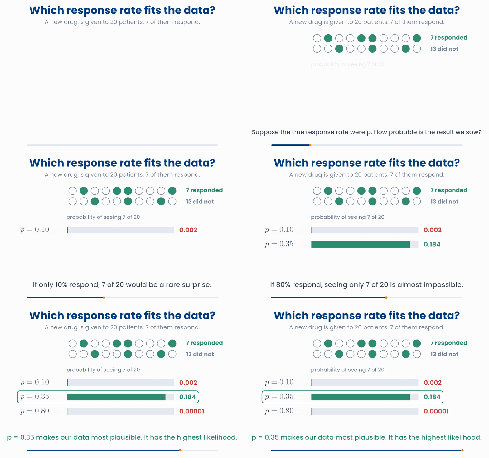
The probability of the observed data, worked out for one value of the parameter, is called the likelihood of that value. We write it \(L(p)\). Here \(L(0.10) = 0.002\), \(L(0.35) = 0.184\) and \(L(0.80) = 0.00001\). The value \(p = 0.35\) makes our data more than 90 times as probable as \(p = 0.10\) does.
Likelihood: the height of the bar you observed
Move p. The top plot shows how many responders the model expects if the rate were p. The orange bar is the result we actually saw. Its height is the likelihood, which is plotted below. Visit many values of p to trace the curve.
So one formula can be read in two directions. This is a key idea:
| What is fixed | What varies | |
|---|---|---|
| Probability (top plot) | the parameter \(p\) | the possible results: 0, 1, …, 20 responders |
| Likelihood (bottom plot) | the data: 7 responders out of 20 | the parameter \(p\) |
A product over patients. The likelihood is built one patient at a time. A responder has probability \(p\). A non-responder has probability \(1 - p\). The patients are independent, so the chance of the whole data set is the product of the chances for each patient. This is the \(\Pi\) from lesson 1.1:
For \(p = 0.35\) this product is 0.0000024. That is the probability of these exact 20 results, patient by patient. The 0.184 in the animation is the probability of 7 responders in any order. It is the same product multiplied by 77,520, the number of different ways to choose which 7 of the 20 respond. That factor does not depend on \(p\), so it never changes which \(p\) is best. Statisticians usually leave it out.
The likelihood is not the probability that p is true
import numpy as np
responded = np.array([0,1,0,0,1,1,0,0,0,1, 0,0,1,0,0,1,0,0,1,0])   # 1 = responded

def likelihood(p):
    chance = np.where(responded == 1, p, 1 - p)   # each patient's probability
    return chance.prod()                          # multiply them all

print(likelihood(0.10))            # 2.5e-08
print(likelihood(0.35))            # 2.4e-06   the largest of the three
print(likelihood(0.35) * 77520) # 0.184 the binomial probability of 7 out of 20Twelve patients take a test drug, and 3 of them get a rash. The model says each patient gets the rash with probability \(q\), independently. Which expression is the likelihood \(L(q)\)?
3 Maximum likelihood
The likelihood gives a score to every possible value of \(p\). The natural choice is the value with the highest score. That value is the maximum likelihood estimate, or MLE. Like every estimate, it wears a hat: \(\hat{p}\), "p hat".
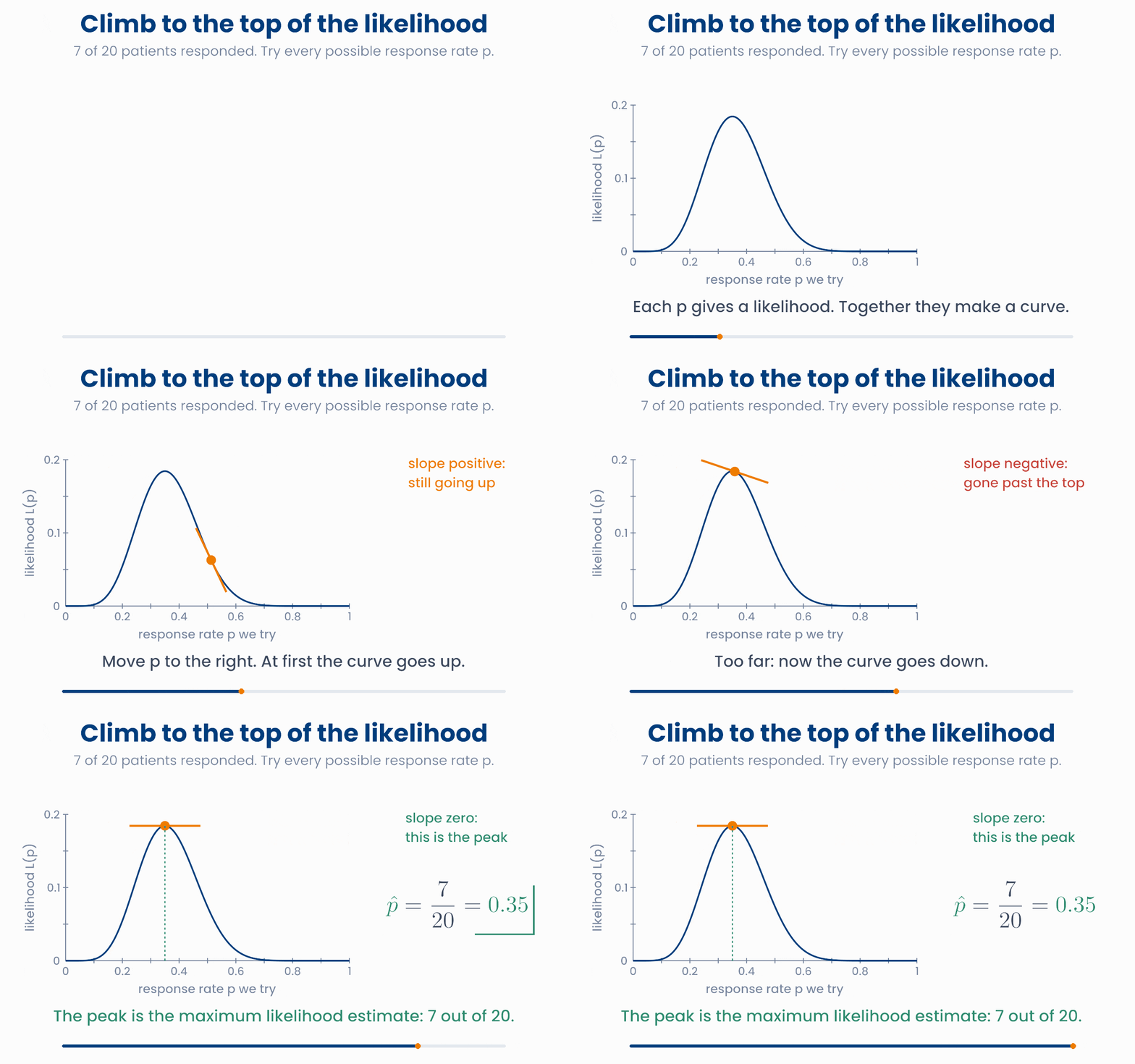
You know from Unit 3 how to find the top of a smooth curve: it is where the slope is zero. For \(k\) responders out of \(n\) patients, this always gives the same answer:
This is the answer you would have guessed. That is reassuring: maximum likelihood is a general method, and in simple cases it agrees with common sense. Its power is that it also works for models where nobody could guess the answer.
A second example: the mean of a lab value. Five patients have a fasting glucose of 5.2, 5.9, 6.4, 5.5 and 6.0 mmol/L. Suppose the values come from a normal distribution with an unknown mean \(\mu\) and, to keep things simple, a known standard deviation of 0.5 mmol/L. For a measured value like this, each patient's part of the likelihood is the height of the normal curve at that patient's value. The likelihood is the product of the five heights.
Slide the bell curve over the patients
Move μ. The orange lines are the heights of the curve at the five patients' values. The likelihood multiplies them. Find the μ that makes the log-likelihood in the lower plot as large as possible.
The best value is \(\hat{\mu} = 5.8\) mmol/L, which is the ordinary mean of the five values. When the curve sits over the middle of the data, every patient gets a good height. Move it away, and some patients land in the thin tail of the curve. Their heights are close to zero, so the whole product collapses.
Why you will care later
import numpy as np
p = np.linspace(0, 1, 1001)          # try 1,001 response rates
L = p**7 * (1 - p)**13               # likelihood of 7 responders and 13 non-responders
print(round(p[np.argmax(L)], 2))     # 0.35  the peak, 7/20

glucose = np.array([5.2, 5.9, 6.4, 5.5, 6.0])
mu = np.linspace(4.5, 7.0, 251)      # try many means
L = [np.prod(np.exp(-(glucose - m)**2 / 0.5)) for m in mu]   # bell heights (SD 0.5), constant left out
print(round(mu[np.argmax(L)], 2)) # 5.8 the mean of the five valuesA screening study tests 80 adults for a gene variant, and 12 of them carry it. The model says each adult carries it with probability \(p\). What is the maximum likelihood estimate \(\hat{p}\)?
4 Log-likelihood
The likelihood multiplies one probability per patient. Every probability is less than 1, so the product shrinks with every patient. For 20 patients it was 0.0000024. For 1,000 patients with 35% responders it is about \(10^{-281}\). A computer cannot store numbers much smaller than about \(10^{-308}\). Below that it loses accuracy, and soon it rounds to exactly 0. Then every value of \(p\) looks equally bad.
The fix is the rule from lesson 1.2: the log of a product is the sum of the logs. So instead of the likelihood we work with the log-likelihood, \(\ln L\):
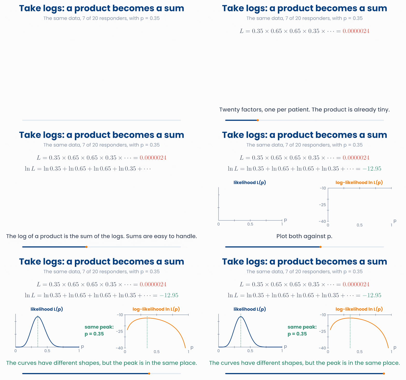
The log-likelihood is a sum, so it does not shrink towards zero: for 1,000 patients it is about \(-647\), an ordinary number. And because the log always goes up when its input goes up, the highest point of \(\ln L\) is at the same \(p\) as the highest point of \(L\). Taking logs changes the height of the hill, but not where its top is.
Why computers add logs instead of multiplying
Increase the number of patients. In every study 35% respond. Blue: the likelihood, multiplied out patient by patient. Orange dashed: the same value found from the sum of logs. Watch the blue line when it reaches the red limit.
Find the peak with the log-likelihood
- \(\ln L(p) = 7 \ln p + 13 \ln(1-p)\).
- Its slope (Unit 3: the derivative of \(\ln p\) is \(1/p\), and of \(\ln(1-p)\) it is \(-1/(1-p)\)) is \(\dfrac{7}{p} - \dfrac{13}{1-p}\).
- Set the slope to zero: \(7(1-p) = 13p\), so \(7 = 20p\) and \(\hat{p} = 7/20 = 0.35\).
Turn it upside down: a loss. Optimisation software usually looks for a minimum, not a maximum. So we flip the sign and use the negative log-likelihood, \(-\ln L\). Now small is good and large is bad, like an error score. A score that the fitting process tries to make as small as possible is called a loss.
Why you will care later
import numpy as np
y = np.array([0] * 1300 + [1] * 700)   # 2,000 patients, 700 responded
p = 0.35
chance = np.where(y == 1, p, 1 - p)    # one probability per patient

print(chance.prod())                   # 0.0       too small: the computer gives up
print(np.log(chance).sum())            # -1294.89  the log-likelihood, no problem
print(-np.log(chance).sum()) # 1294.89 the negative log-likelihood, a lossWhy do statistical programs maximise the log-likelihood instead of the likelihood itself?
5 Least squares
Now a model with two parameters. Eight patients have their age and systolic blood pressure measured. The model is a straight line, as in lesson 1.2:
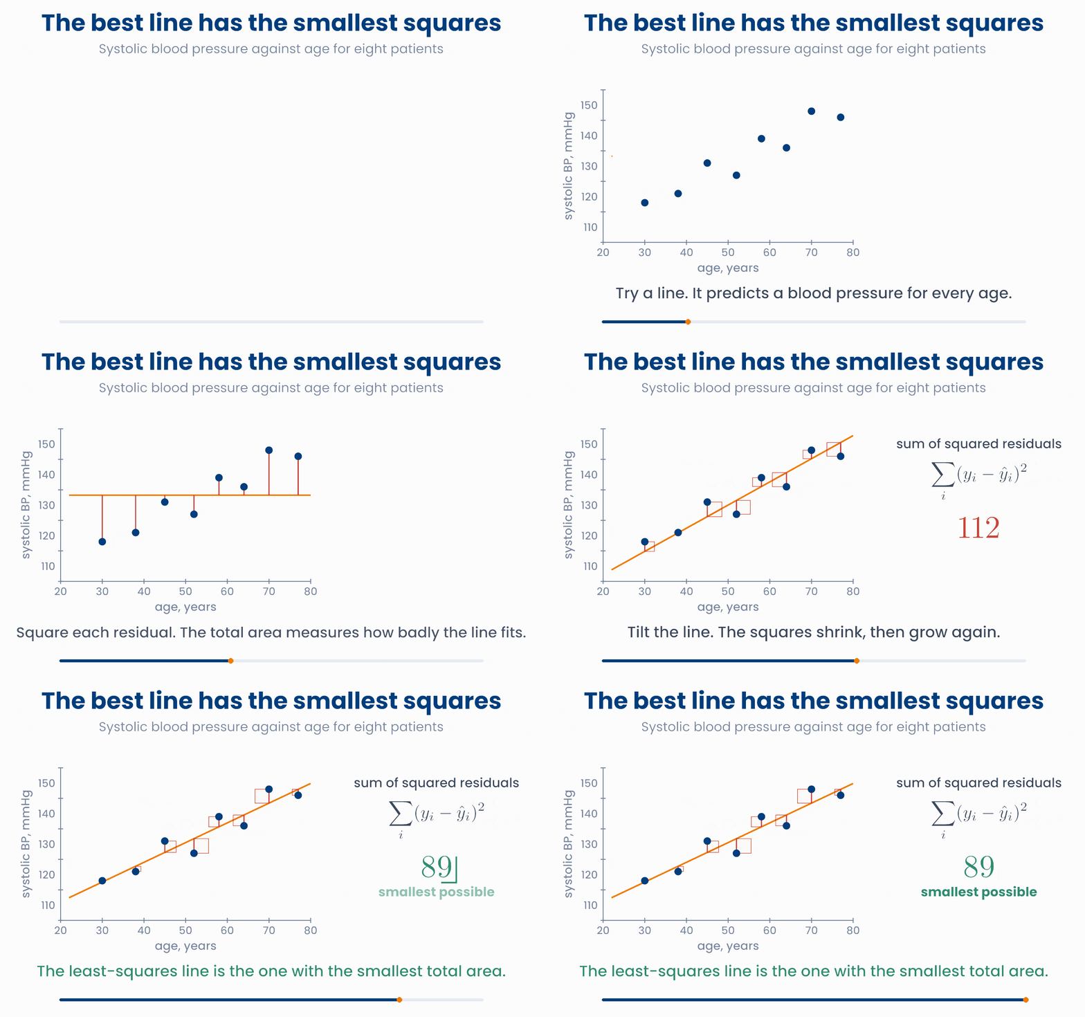
For each patient the line makes a prediction \(\hat{y}_i\). The gap between what was measured and what the line predicts is the residual:
A good line has small residuals. We cannot add them up as they are, because positive and negative residuals cancel. So, as with the variance in lesson 1.1, we square them and add the squares. The result is the sum of squared residuals:
The least-squares line is the line with the smallest SS. You can draw each squared residual as a real square, with the residual as its side. The best line is the one that makes the total area of the squares as small as possible.
Make the squares as small as you can
Change the intercept and the slope. Each red square is one patient's squared residual. Try to make the total area, the sum of squares, as small as possible. Then press the button to see the best line.
The best line here is \(\hat{y} = 98.2 + 0.646 \times \text{age}\), with \(\mathrm{SS} = 88.5\). A flat line at the mean blood pressure gives \(\mathrm{SS} = 847.5\), almost ten times as much. The slope says that, in these patients, blood pressure is about 0.65 mmHg higher for each extra year of age.
You never have to search by hand. For a straight line there is an exact formula, and NumPy applies it in one line. With several inputs (age, BMI, sodium intake…) the same idea fits \(\hat{y} = X\beta\) from Unit 2. This is linear regression.
Why you will care later
import numpy as np
age = np.array([30, 38, 45, 52, 58, 64, 70, 77])
sbp = np.array([118, 121, 131, 127, 139, 136, 148, 146])

slope, intercept = np.polyfit(age, sbp, 1)        # the least-squares line
print(round(intercept, 1), round(slope, 3))       # 98.2 0.646
residuals = sbp - (intercept + slope * age)
print(round((residuals ** 2).sum(), 1))           # 88.5   the smallest possible SS
print(((sbp - sbp.mean()) ** 2).sum()) # 847.5 SS of a flat line at the meanA line predicts systolic blood pressure as \(\hat{y} = 100 + 0.6 \times \text{age}\). A 60-year-old patient has a measured value of 142 mmHg. What is this patient's residual, and how much does the patient add to the sum of squared residuals?
6 Two views, one answer
We now have two rules for "best fit": maximum likelihood and least squares. For a straight line they do not compete. With one extra assumption, they give exactly the same line.
The assumption is about the errors. Suppose each blood pressure is the line plus a random error, and the errors follow a normal distribution with mean 0 and the same standard deviation \(\sigma\) at every age:
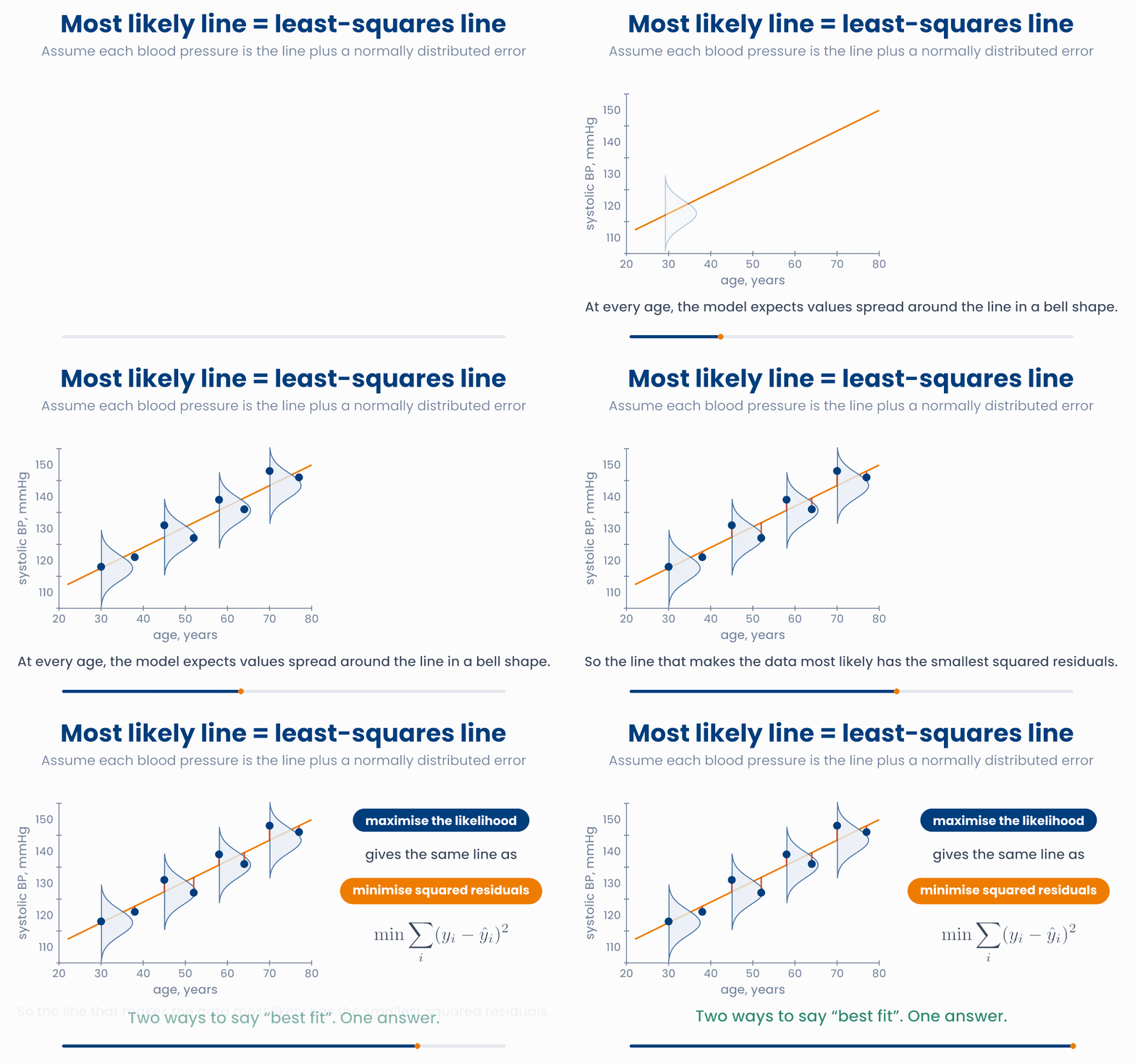
Why are the two rules the same? Each patient's likelihood is the height of the bell curve at their blood pressure. A patient on the line gets the top of the bell. A patient far from the line lands in the tail, where the height is close to zero. In symbols, the log of the bell's height is a constant minus the squared residual divided by \(2\sigma^2\). Add this up over the patients:
So the largest log-likelihood comes from the smallest sum of squared residuals. The most likely line is the least-squares line.
One slider, two scores, one best line
Tilt the line (it always passes through the centre of the data). The middle plot is the sum of squares: smaller is better. The bottom plot is the log-likelihood with normal errors: larger is better. Watch where each one is best.
Fitting is minimising a loss. This is the main message of the lesson. Almost every model in statistics and machine learning is fitted in the same two steps. First, write down a loss: a number that says how badly the model agrees with the data. Then find the parameter values that make the loss as small as possible.
| Model | What it predicts | Loss that is made smallest |
|---|---|---|
| Linear regression | a number, such as blood pressure | sum of squared residuals (the same as the negative log-likelihood with normal errors) |
| Logistic regression | a probability, such as the risk of diabetes | negative log-likelihood, also called log loss or cross-entropy |
| Neural network | either of the above | the same losses, with thousands or millions of parameters |
Why you will care later
import numpy as np
age = np.array([30, 38, 45, 52, 58, 64, 70, 77])
sbp = np.array([118, 121, 131, 127, 139, 136, 148, 146])

for slope in [0.4, 0.646, 0.9]:
    intercept = sbp.mean() - slope * age.mean()     # line through the centre of the data
    r = sbp - (intercept + slope * age)             # residuals
    loglik = (-np.log(4 * np.sqrt(2 * np.pi)) - r**2 / (2 * 4**2)).sum()   # normal errors, SD 4
    print(slope, round((r**2).sum(), 1), round(loglik, 2))
# 0.4    198.7  -24.65
# 0.646  88.5   -21.21   smallest SS and largest log-likelihood
# 0.9 205.6 -24.87Two analysts fit a line of drug clearance against body weight to the same 50 patients. One uses least squares. The other uses maximum likelihood, assuming normal errors with the same standard deviation for every patient. What will they find?
7 Check your understanding
Five short questions on this lesson. Nothing is graded or saved outside this browser. If you choose a wrong option you get a hint, and you can try again.
A model for a blood test has one parameter, \(\mu\). Which sentence describes the likelihood \(L(\mu)\)?
In a trial, 18 of 60 patients have a relapse within a year. Each patient relapses with probability \(p\), independently. Which is the likelihood, and where is its peak?
Two models are fitted to the same 5,000 patients. Model 1 has a log-likelihood of \(-2{,}310\). Model 2 has a log-likelihood of \(-2{,}450\). Which model makes the observed data more likely?
The line \(\hat{y} = 50 + 2x\) is used for three patients with \((x, y) = (10, 72),\ (20, 88)\) and \((30, 113)\). What is the sum of squared residuals?
When the errors are assumed to be normal, why is the line with the largest likelihood also the least-squares line?