

1 Introduction
A research team wants to know the mean systolic blood pressure of adults in Singapore. There are millions of adults. The team cannot measure them all. So it measures 200 people and reports: "the mean is 129.4 mmHg".
That number comes from 200 people. The question was about millions. Two things follow:
- If the team had picked 200 other people, the answer would be a little different.
- So the reported number is not the truth. It is an estimate of the truth, and it carries some uncertainty.
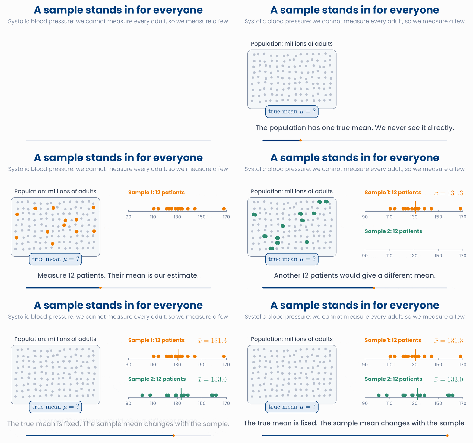
This lesson gives you the words and the pictures for that uncertainty. It does not need new mathematics. You already have the mean and the standard deviation from lesson 1.1, and the normal distribution from lesson 4.2. Here you put them to work.
The second half of the lesson asks a different question about a sample: when one measurement is high, does another measurement tend to be high too? That is the idea of correlation.
What you will be able to do
- Tell a parameter (the truth about a population) from a statistic (what you measured in a sample).
- Explain why a sample mean changes from sample to sample, and use the standard error to say by how much.
- Read "estimate ± 2 standard errors" as a range of plausible values.
- Read a covariance and a correlation \(r\), and know what they cannot tell you.
2 Population and sample
The population is the whole group you want to know about: all adults in a country, all patients with type 2 diabetes, all tumours of one kind. The sample is the part of the population that you measured.
A number that describes the population is called a parameter. It is fixed, but you do not know it. A number that you calculate from the sample is called a statistic. You know it exactly, but it would change if you took another sample.
Formulas keep the two apart by using different letters. Greek letters are for the population. Latin letters, bars and hats are for the sample.
| Quantity | Population (parameter, unknown) | Sample (statistic, measured) |
|---|---|---|
| Mean | \(\mu\) "mu" | \(\bar{x}\) "x bar" |
| Standard deviation | \(\sigma\) "sigma" | \(s\) |
| Proportion | \(p\) | \(\hat{p}\) "p hat" |
(A proportion is a fraction of people, for example the fraction of patients who respond to a drug.)
So when a paper writes \(\bar{x} = 129.4\), it is telling you what was measured. When it writes \(\mu\), it is talking about the true value that nobody can see.
The parameter stays. The statistic moves.
Press the button several times. The curve and the dashed line (the population) never change. The dots and the orange line (your sample) change every time.
In real life you only get the orange numbers
import numpy as np
rng = np.random.default_rng(1)
population = rng.normal(128, 20, size=1_000_000)   # pretend we can see everyone
sample = rng.choice(population, size=200, replace=False)

print(population.mean())     # 128.0  the parameter mu
print(sample.mean())         # 129.4  the statistic x-bar
print(sample.std(ddof=1)) # 19.6 the statistic sA study measures HbA1c in 150 patients with type 2 diabetes from one clinic. It reports a mean of 7.4%. The team wants to learn about all patients with type 2 diabetes in the country. Which statement is correct?
3 Sampling variability
Your sample is only one of very many samples you could have drawn. Each possible sample has its own mean. So the sample mean is itself a quantity that varies. This is called sampling variability.
To see it, imagine that many teams run the same study. Each team measures 25 patients from the same population. Each team reports its own mean.
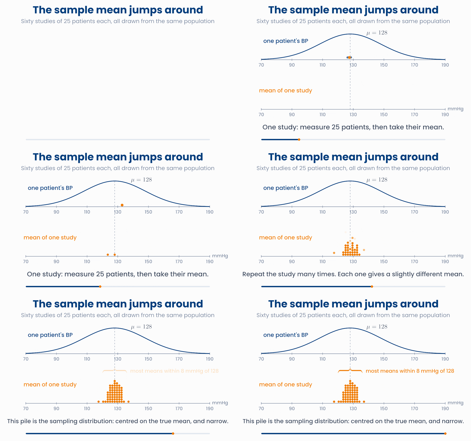
The pile of means has a name. It is the sampling distribution of the mean. Look at three things in it:
- Centre. The means pile up around the true mean \(\mu\). On average, the sample mean is right.
- Spread. The pile is much narrower than the population. A mean of 25 patients varies less than one patient does, because high and low values inside a sample partly cancel.
- Shape. The pile looks like a normal curve. This is the central limit theorem that you met by simulation in lesson 4.2.
Pile up the sample means
Draw samples one at a time, then 200 at once. Then change n. Watch how wide the orange pile is compared with the blue population.
Try \(n = 5\) and then \(n = 100\) in the figure. With more patients in each sample, the means stay closer to \(\mu\). The last tile in the figure, \(\sigma / \sqrt{n}\), predicts how wide the pile will be. The next section explains it.
import numpy as np
rng = np.random.default_rng(2)
studies = rng.normal(128, 20, size=(1000, 25))   # 1000 studies, 25 patients each
means = studies.mean(axis=1)                     # one mean per study

print(means[:5].round(1))    # [127.8 129.1 129.5 124.9 131.6]  they jump around
print(means.mean())          # 128.2  centred on mu
print(means.std(ddof=1)) # 4.07 much less than sigma = 20A team measures serum cholesterol in 40 patients and finds a mean of 5.3 mmol/L. A second team measures 40 other patients from the same population in the same way. What should you expect?
4 Standard error
In a real study you have one sample. You cannot repeat the study a thousand times to see how much the mean jumps around. You do not need to. The spread of the sampling distribution can be worked out from your one sample. It is called the standard error of the mean, written SE.
Read the formula in two parts. If patients differ a lot from each other (large \(s\)), the mean is harder to pin down. If you measure many patients (large \(n\)), it is easier.
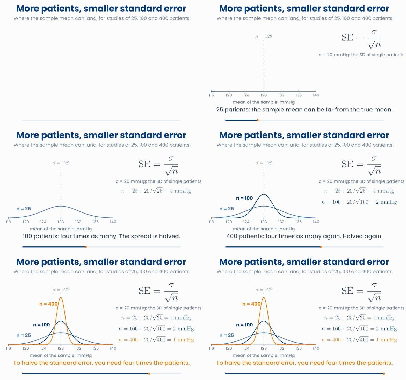
The animation uses the population SD, \(\sigma = 20\) mmHg, because we built that population ourselves. In a real study \(\sigma\) is unknown, so you put the sample SD \(s\) in its place. That is the formula above.
SD and SE answer different questions
Because of the square root, precision is expensive. To halve the standard error you need four times the patients. To make it ten times smaller you need a hundred times the patients.
Four times the patients, half the standard error
Move n. The orange dot is your study. The green dot is a study four times as large. Compare the two standard errors.
What do you do with a standard error? You use it to give a range of plausible values for the true mean. The sample mean is rarely more than about 2 standard errors away from \(\mu\). So the range
will contain \(\mu\) in most studies. This range is called a 95% confidence interval. The name comes from a picture of repeated studies: if 100 teams each ran the study and each built this range, about 95 of the 100 ranges would contain the true mean.
Forty studies, forty intervals
Each bar is one study: its mean ± 2 SE. Blue bars contain the true mean. Red bars miss it. Run new studies several times and watch the percentage. Then change n and watch the width.
One study, one interval
- A study measures \(n = 100\) patients. It finds \(\bar{x} = 126.8\) mmHg and \(s = 21.4\) mmHg.
- Standard error: \(\mathrm{SE} = 21.4 / \sqrt{100} = 2.14\) mmHg.
- Range: \(126.8 \pm 2 \times 2.14\), which is from 122.5 to 131.1 mmHg.
- In words: "Our best estimate of the mean is 126.8 mmHg. Values between about 122 and 131 mmHg are plausible for the true mean."
What the interval does not say
Why you will care later
import numpy as np
rng = np.random.default_rng(3)
x = rng.normal(128, 20, size=100)     # one study of 100 patients

n = len(x)
s = x.std(ddof=1)
se = s / np.sqrt(n)
print(x.mean())                          # 126.8
print(s, se)                             # 21.4  2.14
print(x.mean() - 2 * se, x.mean() + 2 * se) # 122.5 131.1A study of 36 patients finds a standard deviation of \(s = 12\) mmHg, so \(\mathrm{SE} = 12 / \sqrt{36} = 2\) mmHg. The team wants a standard error of 1 mmHg. About how many patients do they need?
5 Covariance: moving together
So far we looked at one measurement at a time. Precision health is mostly about how measurements relate to each other. Does blood pressure rise with age? Does drug clearance rise with body weight? Does the expression of one gene go up when another goes down?
Take six patients. For each one we have the age, \(x_i\), and the systolic blood pressure, \(y_i\). Plot one dot per patient. Then draw the mean age and the mean blood pressure. The two lines cut the plot into four parts.
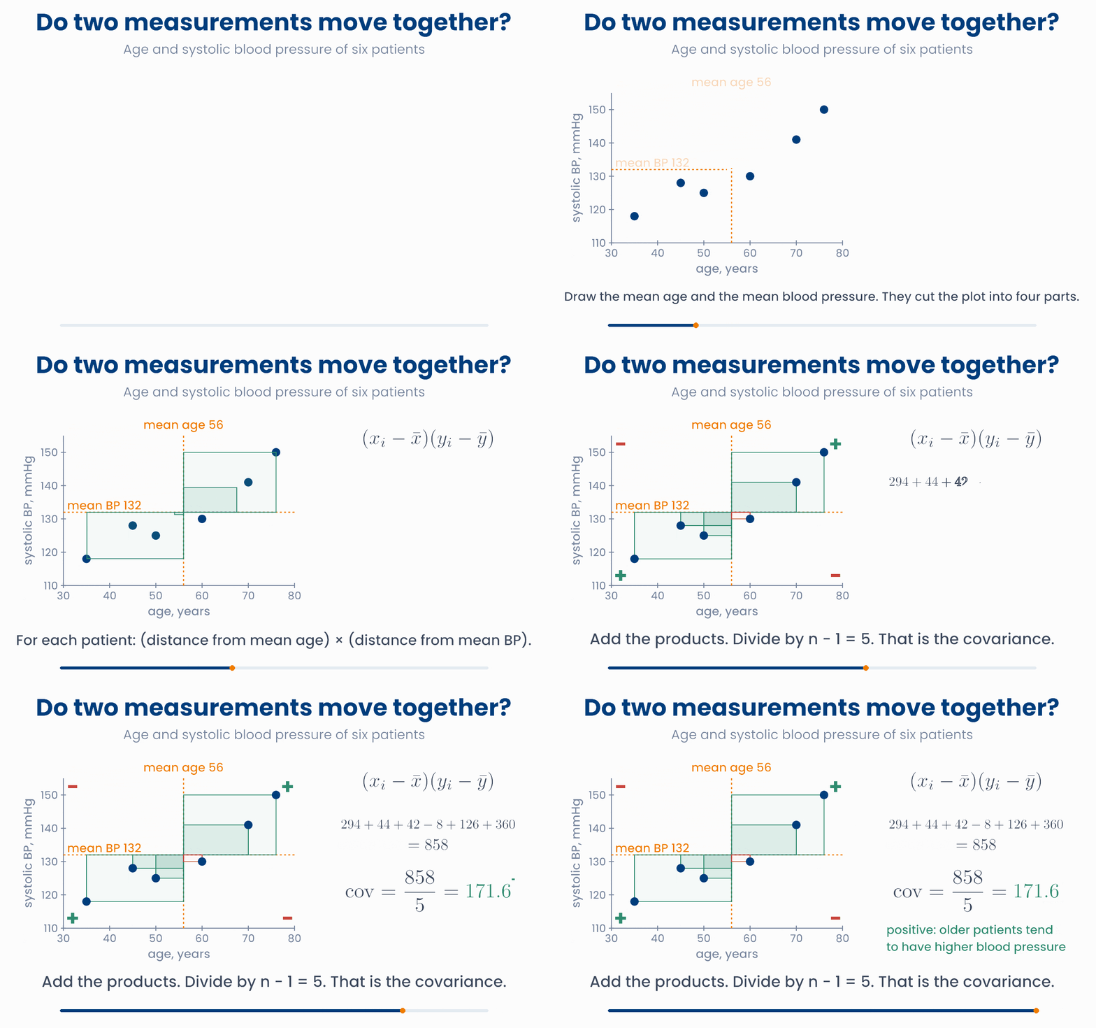
For each patient, multiply two deviations: the distance from the mean age, and the distance from the mean blood pressure.
- Older than average and higher pressure than average: plus times plus. The product is positive.
- Younger than average and lower pressure than average: minus times minus. The product is also positive.
- One above its mean and the other below: plus times minus. The product is negative.
The covariance is the average of these products. As with the variance, we divide by \(n - 1\).
Compare this with the variance from lesson 1.1. There each patient gave a square, \((x_i - \bar{x})^2\). Here each patient gives a rectangle: one side from \(x\), one side from \(y\). The variance is the covariance of a measurement with itself.
Each patient adds a rectangle
Drag any dot. Green rectangles count as positive, red as negative. Try to make the covariance zero, then negative. Then switch age to months.
Two things to read from a covariance:
- The sign matters. Positive: the two measurements tend to be high together and low together. Negative: when one is high, the other tends to be low. Near zero: no clear straight-line pattern.
- The size is hard to read. The covariance here is 171.6 "mmHg × years". If you record age in months, the same patients give 2059.2. Nothing about the patients changed. So you cannot say whether 171.6 is a strong link or a weak one.
Why you will care later
import numpy as np
age = np.array([35, 45, 50, 60, 70, 76])
sbp = np.array([118, 128, 125, 130, 141, 150])

products = (age - age.mean()) * (sbp - sbp.mean())
print(products)                       # [294.  44.  42.  -8. 126. 360.]
print(products.sum() / (len(age) - 1))  # 171.6
print(np.cov(age, sbp)[0, 1])         # 171.6   the same thing in one step
print(np.cov(age * 12, sbp)[0, 1]) # 2059.2 age in months: same patients, new numberIn a group of adults, people who exercise more hours per week tend to have a lower resting heart rate. What can you say about the covariance between hours of exercise and resting heart rate?
6 Correlation
The covariance has a problem: its size depends on the units. The fix is to divide by the two standard deviations. The units cancel. What is left is the correlation coefficient, written \(r\).
For the six patients: \(s_x = 15.56\) years, \(s_y = 11.58\) mmHg, so \(r = 171.6 / (15.56 \times 11.58) = 0.95\). With age in months you get the same 0.95.
The correlation always lies between \(-1\) and \(+1\):
- \(r = +1\): all dots lie exactly on a rising straight line.
- \(r = -1\): all dots lie exactly on a falling straight line.
- \(r = 0\): no straight-line pattern at all.
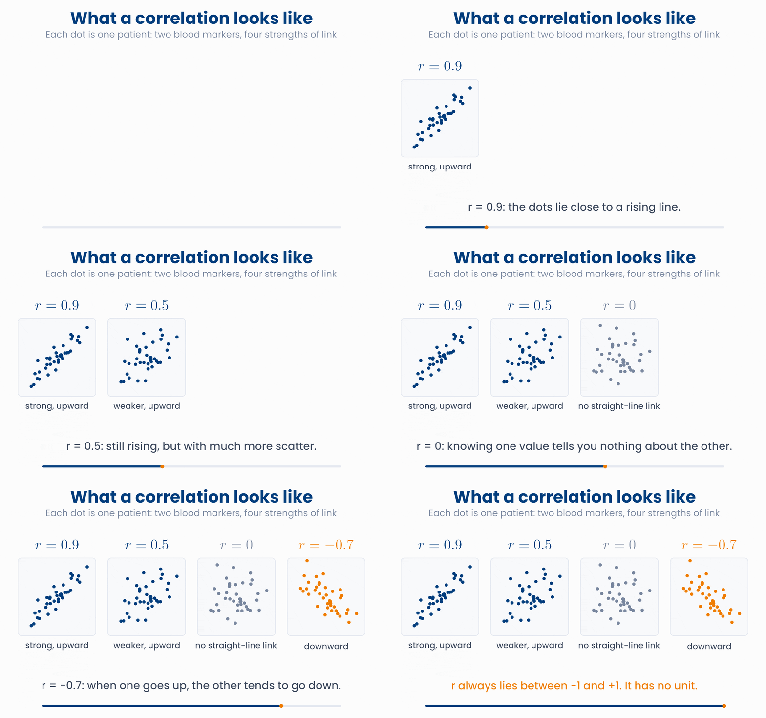
Set r and see the cloud
Move the slider from −1 to +1. Find the values 0.9, 0.5, 0 and −0.7. How tight does the cloud have to be before you would call the link strong?
The correlation is useful, but it is easy to read too much into it. Keep three warnings in mind.
1. It only measures straight-line association. A drug can work best at a medium dose and worse at low and high doses. Dose and effect are then strongly related, but the dots form an arch, not a line, and \(r\) can be close to 0. Always look at the scatter plot, not only at \(r\).
2. It is sensitive to outliers. One unusual patient can create a correlation that is not there for anyone else, or hide one that is.
One patient can change r
Drag the orange patient. Put it far up on the right, then far down on the right, then inside the blue cloud. Watch the two values of r.
3. Correlation is not causation. Two measurements can move together without one causing the other. A common reason is a third factor that drives both. It is called a confounder.
A confounder in a hospital
- Hospital records show: patients who were admitted to the intensive care unit (ICU) died more often than patients who were not.
- So "ICU admission" and "death" are positively correlated.
- Does intensive care cause death? No. A third factor, how ill the patient is, drives both. Very ill patients are sent to the ICU, and very ill patients are more likely to die.
- To learn what the ICU itself does, you must compare patients who are equally ill. A correlation alone cannot do that.
Why you will care later
import numpy as np
age = np.array([35, 45, 50, 60, 70, 76])
sbp = np.array([118, 128, 125, 130, 141, 150])

cov = np.cov(age, sbp)[0, 1]
print(cov / (age.std(ddof=1) * sbp.std(ddof=1)))   # 0.953  from the formula
print(np.corrcoef(age, sbp)[0, 1])                 # 0.953  in one step
print(np.corrcoef(age * 12, sbp)[0, 1]) # 0.953 units do not matterA study of a sedative plots dose against a "comfort score" for 60 patients. Comfort is low at small doses, highest at medium doses and low again at large doses. The correlation is \(r = 0.02\). What is the best conclusion?
7 Check your understanding
Five short questions on this lesson. Nothing is graded or saved outside this browser. If you choose a wrong option you get a hint, and you can try again.
A paper states: "We assume the tumour diameters have mean \(\mu\) and standard deviation \(\sigma\). In our 80 patients we found \(\bar{x} = 2.9\) cm and \(s = 1.1\) cm." Which symbols stand for values that the team actually measured?
A report on 400 patients gives the fasting glucose as "mean 5.8 mmol/L, SD 1.2, SE 0.06". Which sentence uses these numbers correctly?
A pilot study of 100 patients has a standard deviation of 30 units, so the standard error of the mean is 3 units. The full study will have 400 patients. What standard error do you expect, if the SD stays the same?
Body weight and drug clearance are measured in 50 patients. With weight in kilograms the covariance is 4.2. A colleague records the weight in grams. What happens?
In a group of older adults, the number of different medicines a person takes each day is positively correlated with the number of falls per year (\(r = 0.4\)). Which conclusion is justified by this alone?