

1 Introduction
A patient walks into the clinic. Before the nurse measures her blood pressure, you do not know the number. But you do know a lot about it. It will almost certainly be between 90 and 180 mmHg, and values near 120 are far more common than values near 170.
A random variable is a number we have not measured yet, together with what we know about which values are likely. For example:
- the systolic blood pressure of the next patient, in mmHg;
- the number of patients, out of 20 in a trial arm, who respond to a new drug;
- the number of emergency admissions in the next hour;
- the length of stay of the next patient admitted to a ward, in days.
We write a random variable with a capital letter, such as \(X\). A small letter, such as \(x\), is one value it could take. So \(P(X = 3)\) reads "the probability that \(X\) turns out to be 3". Once you have measured, the random variable has become one plain number: a data point.
The list of values a random variable can take, with how likely each one is, is called its distribution. A distribution is the pattern you would see if you measured many, many patients. This lesson introduces the few distributions that you will meet again and again in health data.
What you will be able to do
- Tell a discrete random variable from a continuous one, and read a bar chart or a density curve as a distribution.
- Calculate an expected value \(E[X]\), and say what the variance and standard deviation measure.
- Recognise when a count follows a binomial or a Poisson distribution.
- Use the normal distribution, the 68–95–99.7 rule and z-scores on a lab value.
- Explain, with a simulation, why averages of many patients behave so well: the law of large numbers and the central limit theorem.
2 Random variables and distributions
Random variables come in two kinds.
- A discrete random variable takes separate values that you can list: 0, 1, 2, 3, … Counts are discrete: GP visits in a year, responders in a trial, mutations in a gene.
- A continuous random variable can take any value in a range, such as 5.37 or 5.3712. Measurements are continuous: blood pressure, fasting glucose, weight, the time until an event.
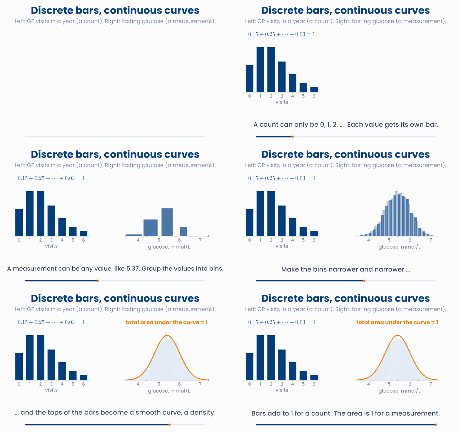
For a discrete variable, the distribution gives a probability to each value. You draw it as bars. The bars must add to 1, because the variable must take one of its values. Here is the number of GP visits in a year for adults in one practice:
| visits \(x\) | 0 | 1 | 2 | 3 | 4 | 5 | 6 |
|---|---|---|---|---|---|---|---|
| \(P(X = x)\) | 0.15 | 0.25 | 0.25 | 0.17 | 0.10 | 0.05 | 0.03 |
A person has only one number of visits, so different values are mutually exclusive, and you can add bars. For example \(P(X \ge 3) = 0.17 + 0.10 + 0.05 + 0.03 = 0.35\).
For a continuous variable, the chance of one exact value is zero: nobody has a glucose of exactly 5.4000000… mmol/L. Instead we ask about ranges. The distribution is a smooth curve called the probability density. As you saw in Unit 3, the probability of a range is the area under the density over that range, and the total area under the curve is 1.
A histogram of many people becomes a density
Make the bins narrower and measure more people. Tick the box to see the density curve. Compare the fraction of people between 5.6 and 7.0 mmol/L with the area under the curve.
Why you will care later
import numpy as np
visits = np.arange(7)                      # GP visits in a year: 0, 1, ..., 6
p = np.array([0.15, 0.25, 0.25, 0.17, 0.10, 0.05, 0.03])
print(p.sum())                 # 1.0   the bars add to 1
print(p[visits >= 3].sum())    # 0.35  P(X >= 3)

rng = np.random.default_rng(1)
glucose = rng.normal(5.4, 0.6, size=100_000)       # fasting glucose, mmol/L
print(((glucose >= 5.6) & (glucose < 7.0)).mean()) # 0.36322 close to the area, 0.366Which of these is a continuous random variable?
3 Expectation and variance
Follow many patients with heart failure for a year and count their hospital admissions. Let \(X\) be the number for one patient. Its distribution is: 0 admissions with probability 0.50, 1 with 0.30, 2 with 0.15 and 3 with 0.05.
What is the average number of admissions per patient? Think of 100 patients. 50 have none, 30 have one, 15 have two and 5 have three. That is \(0 + 30 + 30 + 15 = 75\) admissions, or 0.75 per patient. Dividing by 100 at each step turns the counts into probabilities:
\(E[X]\) is the expected value, or the mean, of the random variable. It is often written \(\mu\). It is the long-run average over many patients. It need not be a value that \(X\) can take: no patient has 0.75 admissions. Notice the sigma from Unit 1. It is an average where each value is weighted by how often it happens, \(p(x)\).
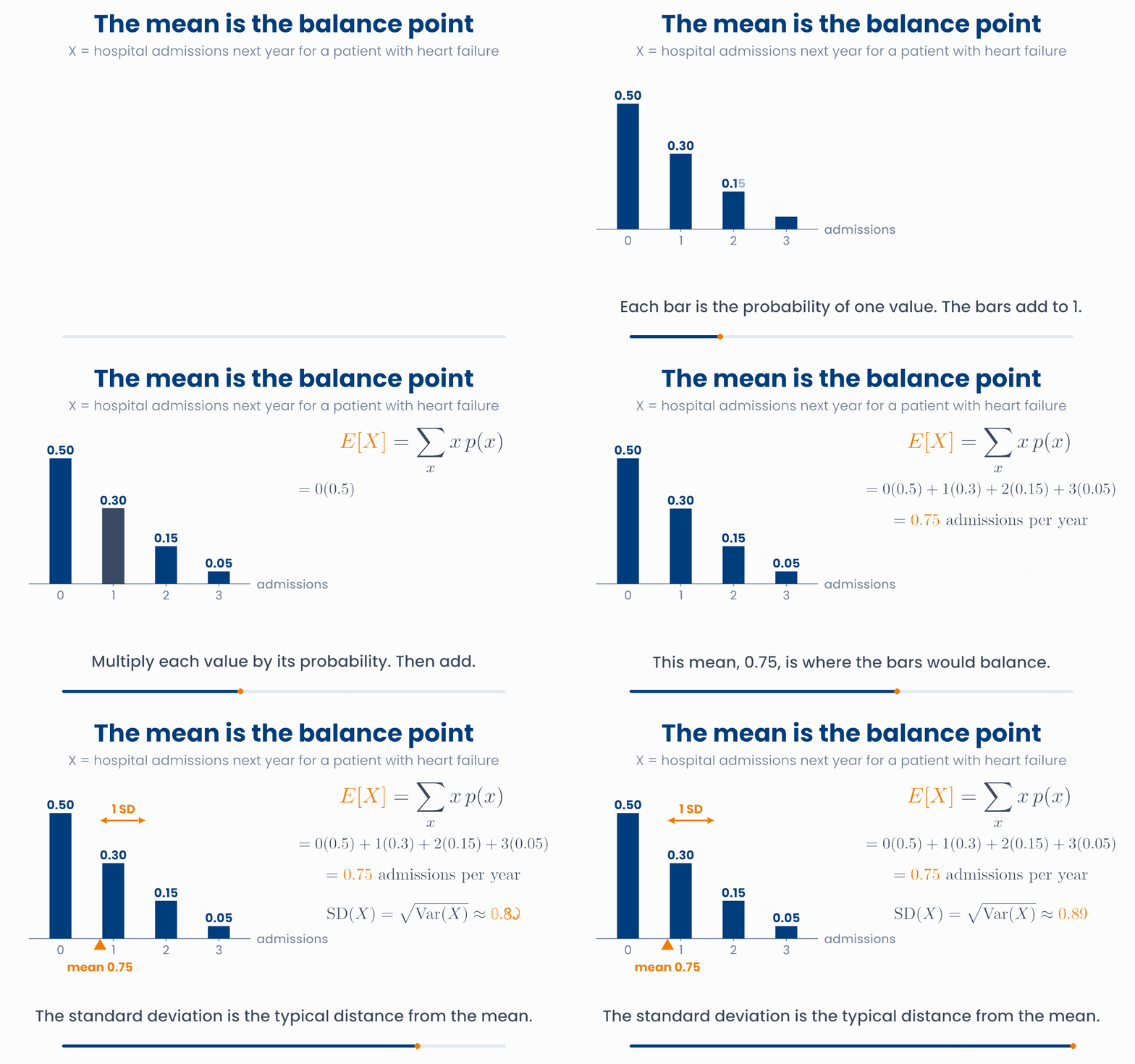
Picture the bars as weights standing on a ruler. The mean is the point where the ruler would balance. A long tail to the right pulls the balance point to the right.
The mean says where the distribution is centred. The variance says how spread out it is. It is the expected squared distance from the mean. The standard deviation (SD) is the square root of the variance, so it is back in the original units. Read the SD as the typical distance of a patient from the mean.
For the admissions, \(\mathrm{Var}(X) = 0.7875\) and \(\mathrm{SD}(X) \approx 0.89\) admissions. These are the same ideas as the sample mean and variance in lesson 1.1. There, each of the \(n\) patients had the weight \(1/n\). Here, each value has the weight \(p(x)\). For a continuous variable the sum becomes an integral, but the meaning is the same.
The mean is where the bars balance
Drag any bar up or down to change how many of the patients had that number of admissions. The orange triangle is the mean (the balance point); the arrows show one SD on each side.
Why you will care later
import numpy as np
x = np.array([0, 1, 2, 3])               # admissions next year
p = np.array([0.50, 0.30, 0.15, 0.05])   # their probabilities

mu = (x * p).sum()                       # E[X] = sum of x p(x)
var = ((x - mu) ** 2 * p).sum()          # Var(X)
print(mu, var.round(4), np.sqrt(var).round(3))   # 0.75 0.7875 0.887

rng = np.random.default_rng(2)
patients = rng.choice(x, size=100_000, p=p)   # 100,000 simulated patients
print(patients.mean()) # 0.75221, the long-run average is close to 0.75\(X\) is the number of doses of a drug that a patient misses in a week: 0 with probability 0.6, 1 with probability 0.3, and 2 with probability 0.1. What is \(E[X]\)?
4 Bernoulli and binomial
The simplest random variable has only two values. A patient responds to a drug (1) or does not (0). If the chance of response is \(p\), then \(P(X = 1) = p\) and \(P(X = 0) = 1 - p\). This is a Bernoulli random variable. Its mean is \(0(1-p) + 1 \cdot p = p\), and its variance is \(p(1-p)\).
Now treat \(n\) patients. Each one responds with the same chance \(p\), and one patient's response does not affect another's: they are independent. The number of responders \(X\) has a binomial distribution, written \(X \sim \text{Binomial}(n, p)\). The sign \(\sim\) reads "has the distribution".
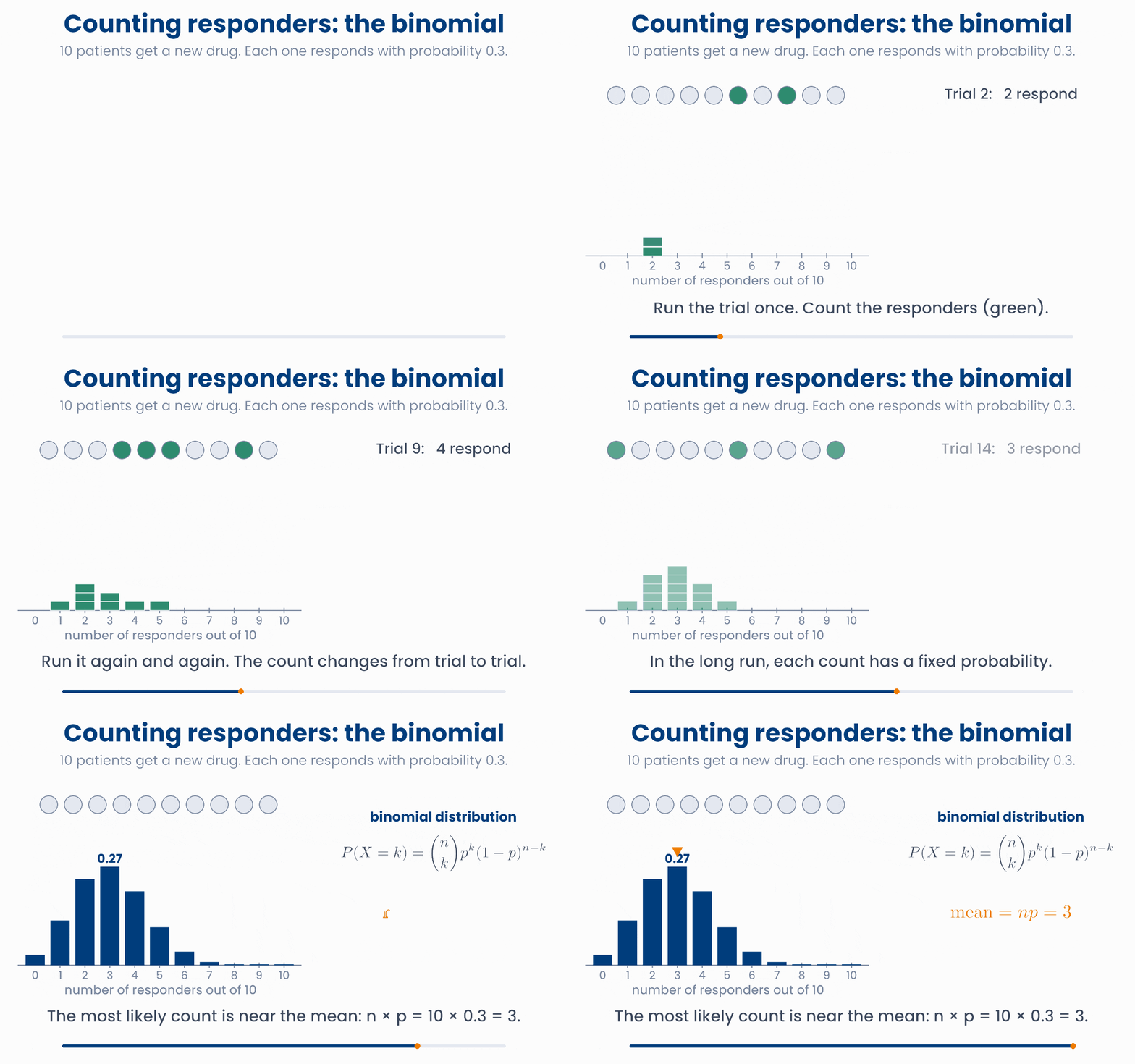
Read it from the inside out, as in Unit 1:
- \(p^k\): \(k\) particular patients all respond. They are independent, so multiply \(p\) by itself \(k\) times.
- \((1-p)^{n-k}\): the other \(n - k\) patients all do not respond.
- \(\binom{n}{k}\), read "\(n\) choose \(k\)": the number of different ways to pick which \(k\) of the \(n\) patients are the responders. For \(n = 10\) and \(k = 3\) there are 120 ways.
For 10 patients with \(p = 0.3\): \(P(X = 3) = 120 \times 0.3^3 \times 0.7^7 \approx 0.267\). The chance that nobody responds is \(0.7^{10} \approx 0.028\).
The mean and variance of a binomial are \(n\) times those of one patient:
For 10 patients with \(p = 0.3\), the mean is 3 responders and the SD is \(\sqrt{2.1} \approx 1.45\) responders.
The shape of the binomial changes with n and p
Change the number of patients and the chance that each one responds. The orange bars are the outcomes with at least k responders; their total is shown below.
Try a \(p\) near 0 or near 1. The bars are lopsided, because the count cannot go below 0 or above \(n\). Then try a large \(n\): the shape becomes a symmetric bell. You will meet that bell again in section 6.
Why you will care later
import numpy as np
rng = np.random.default_rng(0)
x = rng.binomial(n=10, p=0.3, size=100_000)   # 100,000 trial arms of 10 patients
print(x.mean())          # 2.99949  close to n p = 3
print(x.var())           # 2.10283  close to n p (1 - p) = 2.1
print((x == 3).mean()) # 0.26779 close to P(X = 3) = 0.267A new drug works in 20% of patients. It is given to 50 patients, who respond independently. What is the expected number of responders?
5 The Poisson distribution
Some counts have no fixed number of patients behind them. How many emergency admissions will arrive in the next hour? How many serious adverse events happen per 1000 patient-years of treatment? How many sequencing reads fall on a gene? There is no \(n\) here, only a stretch of time or space in which events happen at random.
Suppose events happen independently of each other, at a steady average rate \(\lambda\) (the Greek letter lambda) per window. Then the count \(X\) in one window has a Poisson distribution:
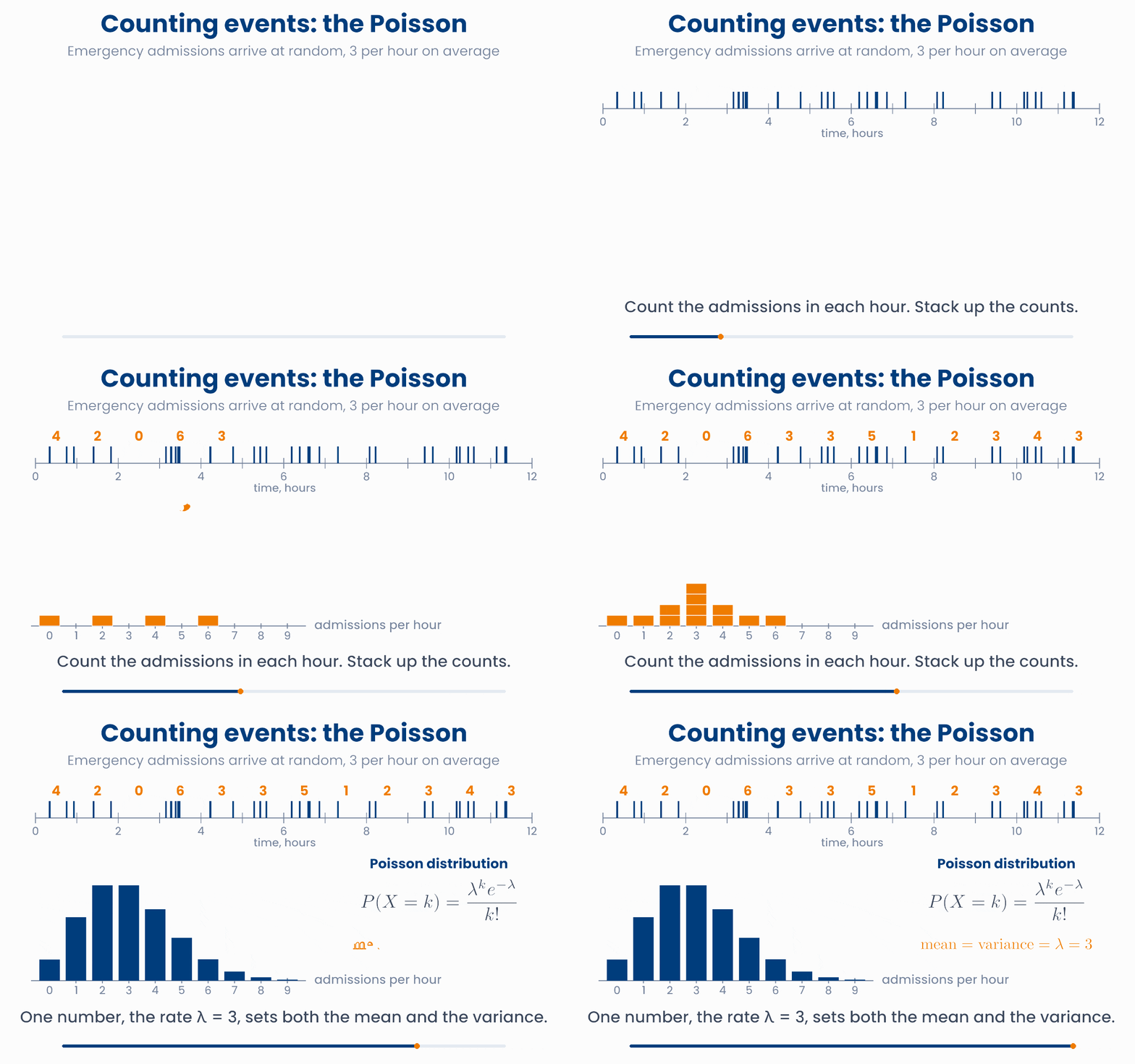
For admissions with \(\lambda = 3\) per hour, \(P(X = 0) = e^{-3} \approx 0.050\): in about 1 hour in 20, nobody arrives. \(P(X = 3) \approx 0.224\). The chance of more than 5 admissions in one hour is about 0.084.
The Poisson distribution has a special property. One number, \(\lambda\), sets both the centre and the spread:
Poisson counts: one rate sets the whole shape
Change the average rate of admissions per hour. Then set how many admissions the team can handle in one hour. Orange bars are the hours when more patients arrive than that.
Here is another example. A drug causes a serious adverse event at a rate of 2 per 1000 patient-years. A study follows its patients for 1000 patient-years in total. The number of events is Poisson with \(\lambda = 2\), so the chance of seeing no events at all is \(e^{-2} \approx 0.14\). A small study that sees no adverse events therefore cannot show that a drug is safe.
Why you will care later
import numpy as np
rng = np.random.default_rng(0)
x = rng.poisson(lam=3, size=100_000)   # admissions in 100,000 separate hours
print(x.mean(), x.var())               # 2.99664 2.99311  mean and variance are both close to 3
print((x > 5).mean()) # 0.0838 P(more than 5 in an hour) is about 0.084A ward records falls among its patients. On average there are 2 falls per month, and the count per month follows a Poisson distribution. What is the variance of the number of falls in a month?
6 The normal distribution
Many measurements in a healthy population pile up in a symmetric bell shape: height, systolic blood pressure, and many lab values (some only after taking logs, as in Unit 1). This bell is the normal distribution, also called the Gaussian. Two numbers describe it completely. The mean \(\mu\) says where the centre is. The standard deviation \(\sigma\) says how wide it is. We write \(X \sim N(\mu, \sigma^2)\).
The shape is always the same bell. So if you measure distances in SDs from the mean, the areas are always the same. This gives the 68–95–99.7 rule.
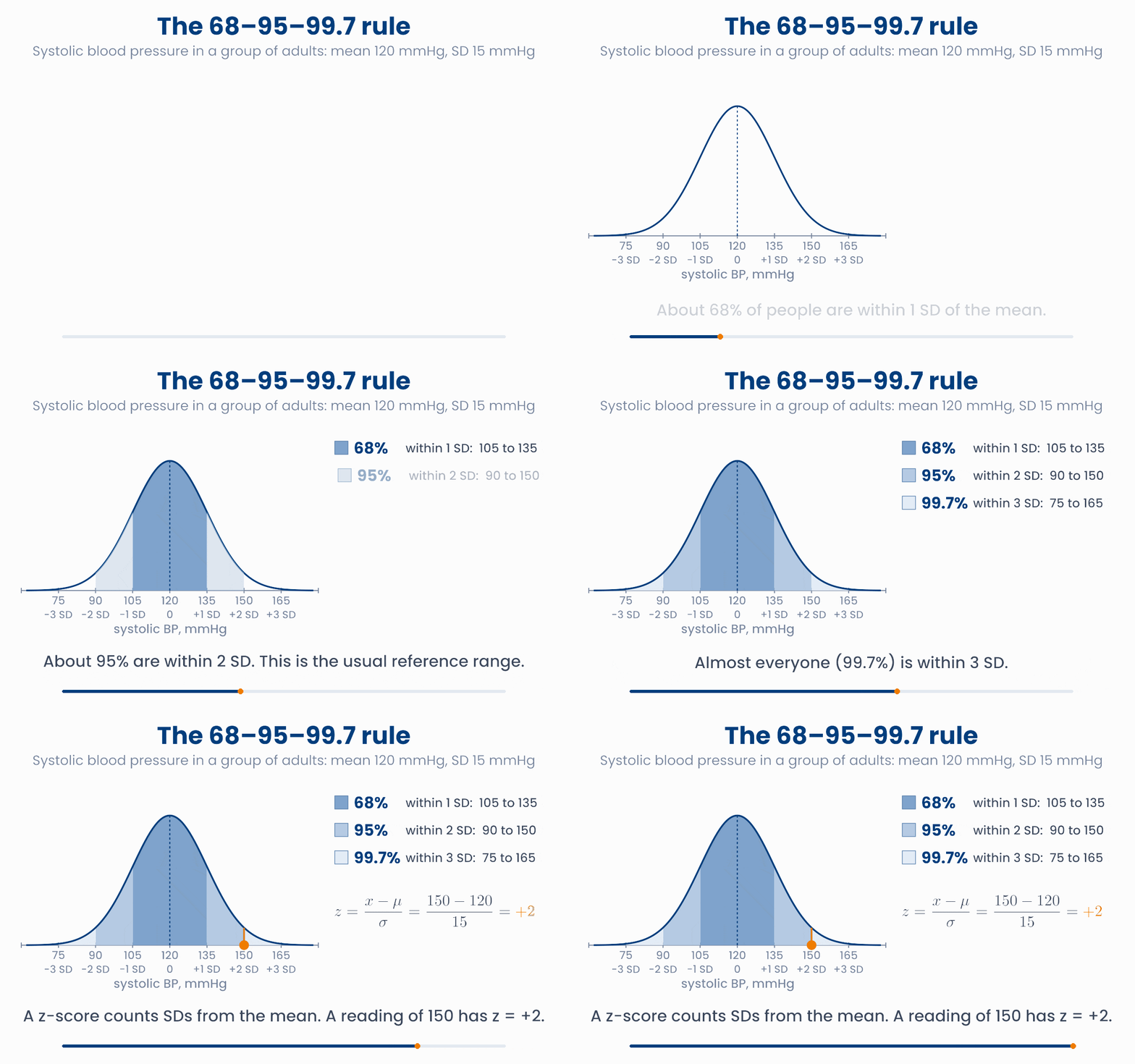
For systolic blood pressure with \(\mu = 120\) and \(\sigma = 15\) mmHg, about 68% of adults lie between 105 and 135 mmHg, about 95% between 90 and 150 mmHg, and almost all (99.7%) between 75 and 165 mmHg.
A z-score says how many SDs a value lies from the mean:
A blood pressure of 150 mmHg has \(z = (150 - 120)/15 = +2\). A z-score of −1 is one SD below the mean. z-scores put different lab tests on one common scale: "2 SDs above the mean" means the same rarity for any normally distributed measurement.
Probability is the area between two limits
Drag the orange limits on the plot, or press a button. Change the mean and the SD and watch the area and the z-scores.
A laboratory reference range is usually the central 95% of healthy people, \(\mu \pm 1.96\sigma\), which is close to \(\mu \pm 2\sigma\). So, by design, 1 healthy person in 20 falls outside it. Order 20 independent tests for a healthy person, and the chance that all 20 come back "normal" is only \(0.95^{20} \approx 0.36\). This is the false alarm problem from Unit 1.
Why you will care later
import numpy as np
rng = np.random.default_rng(0)
sbp = rng.normal(120, 15, size=100_000)       # systolic BP, mmHg
print(((sbp > 90) & (sbp < 150)).mean())      # 0.9546  within 2 SD: about 95%
z = (150 - 120) / 15
print(z)                                      # 2.0
print((sbp > 140).mean()) # 0.09029 about 9% are above 140 mmHgIn healthy adults, HbA1c has a mean of 5.4% and an SD of 0.3%. A patient's HbA1c is 6.0%. What is the z-score?
7 Averages: large numbers and the bell curve
Length of stay in hospital is very uneven. Most patients go home within a few days, but a few stay for weeks. The distribution is skewed: it has a long tail to the right. Suppose the true mean stay on a ward is 5 days, with an SD of about 3.5 days. What happens when we average over many patients?
The law of large numbers. As you include more and more patients, the sample mean settles down on the true mean. Single patients jump around. Their running average does not.
The running mean settles on the true mean
Press Play to admit patients one after another. Each grey dot is one patient's stay; the blue line is the mean of everyone so far. Start again to see a different set of patients.
The central limit theorem. Now take many separate samples of 30 patients, and work out the mean stay of each sample. Each sample gives a slightly different mean. Pile up these means in a histogram.
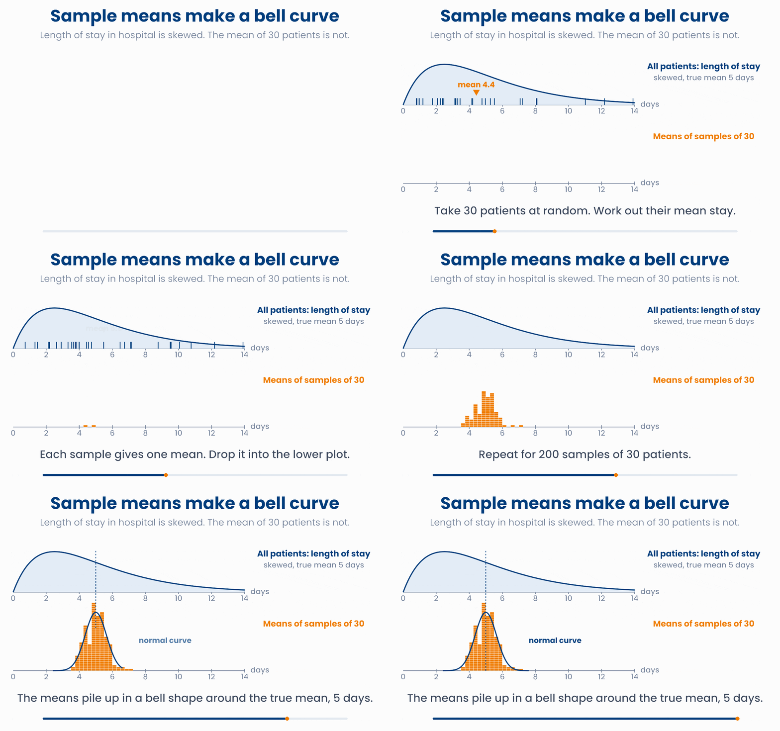
Two things happen. The means centre on the true mean, 5 days. And their histogram is a symmetric bell, even though single stays are skewed. This is the central limit theorem (CLT): the mean of many independent values has an approximately normal distribution, whatever the shape of the single values, as long as the sample is large enough.
Means of samples become bell-shaped
Choose the population and the number of patients in each sample. Then draw more samples. Grey dashed: single patients. Orange bars: the means of the samples. Blue: the normal curve that the central limit theorem predicts.
Use the widget to see the three points that matter:
- With \(n = 1\), each "sample mean" is just one patient. The histogram is as skewed as the data.
- As \(n\) grows, the histogram becomes a bell. For length of stay, \(n = 30\) is already close.
- As \(n\) grows, the bell also becomes narrower: means of larger samples vary less. Unit 5 gives this spread a name, the standard error, and shows how to calculate it.
Key idea
Why you will care later
import numpy as np
rng = np.random.default_rng(4)
stay = rng.gamma(shape=2, scale=2.5, size=(2000, 30))   # 2000 samples of 30 patients, days
means = stay.mean(axis=1)                                # one mean per sample
print(stay.mean().round(2), means.mean().round(2))      # 5.02 5.02  both centre near 5 days
print(stay.std().round(2), means.std().round(2))        # 3.53 0.63  means vary far less

one = rng.gamma(shape=2, scale=2.5, size=1000)          # law of large numbers
print(one[:10].mean().round(2), one[:100].mean().round(2), one.mean().round(2)) # 5.69 4.6 5.07Which statement is the central limit theorem?
8 Check your understanding
Five short questions on this lesson. Nothing is graded or saved outside this browser. If you choose a wrong option you get a hint, and you can try again.
The number of hospital admissions next year for a patient is 0 with probability 0.5, 1 with probability 0.3, and 2 or more with probability \(q\). What is \(q\)?
A study reports that the expected number of adverse events per patient is 0.4. What does this mean?
Which distribution best describes the number of patients, out of 30 vaccinated children, who develop a fever? Assume each child has the same chance and children do not affect each other.
Serum sodium in healthy adults is roughly normal, with a mean of 140 and an SD of 2.5 mmol/L. About what fraction of healthy adults lie between 135 and 145 mmol/L?
You draw many samples of patients' lengths of stay, first with 10 patients per sample and then with 100. How does the histogram of the sample means change?