

1 Introduction
A woman aged 50 joins a screening programme for a disease. The test is a good one. It finds 90% of the people who have the disease, and it clears 90% of the people who do not. Her result comes back positive. What is the chance that she has the disease?
Make a guess before you read on. The disease affects 1 in 100 of the people screened. About how likely is it that she has the disease?
Many people answer "90%". In studies, many doctors gave that answer too. The true answer depends on how common the disease is. When 1 person in 100 has it, the chance is only about 8%. By the end of this lesson you will see why, and you will be able to work it out yourself.
Medicine is full of decisions made under uncertainty. Will this patient respond to the drug? Does this scan show a tumour? Is this result a real signal or a false alarm? Probability is the language for these questions. It puts a number between 0 and 1 on how likely something is.
In this lesson we always think of a probability as a proportion of people. Picture a crowd of 100 or 1000 patients and ask: how many of them? Counting people like this is called using natural frequencies. It makes even Bayes' theorem easy to follow.
What you will be able to do
- Write a probability as a proportion of people, and use \(P(\text{not } A) = 1 - P(A)\).
- Read \(P(A \mid B)\) as "among those with \(B\), the fraction with \(A\)", and see why \(P(A \mid B)\) and \(P(B \mid A)\) are different.
- Say when two events are independent, and when you may multiply their probabilities.
- Build the 2×2 table of a diagnostic test from its sensitivity, its specificity and the prevalence.
- Use Bayes' theorem to turn sensitivity into the chance of disease after a positive test.
2 Probability as a proportion
A health screening event sees 100 adults. 25 of them have high blood pressure. Now choose one of the 100 adults at random, so that every adult has the same chance to be chosen. How likely is it that this person has high blood pressure?
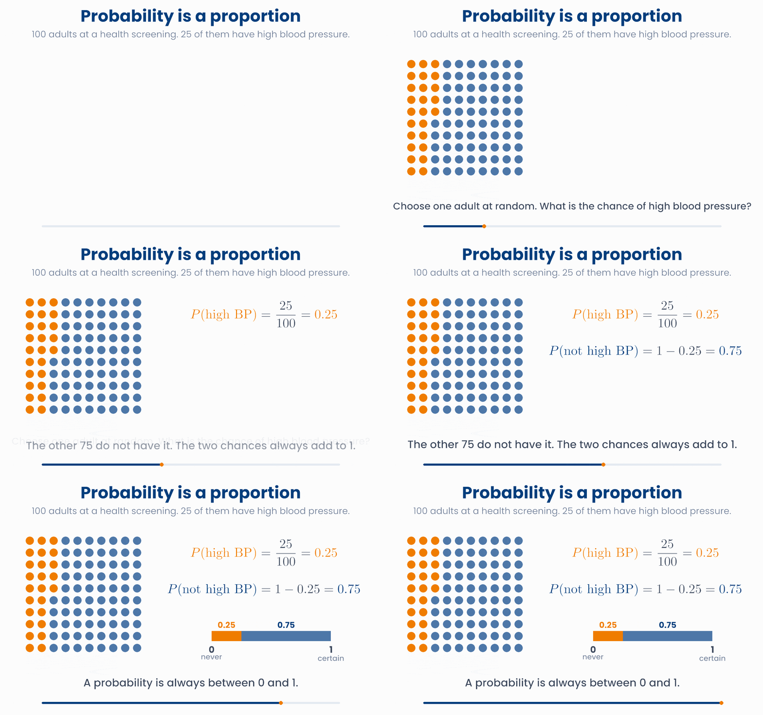
The answer is 25 out of 100:
Here "high BP" is an event: something that is either true or false for each person. \(P(\text{high BP})\) is its probability. Read it as "the probability of high blood pressure". For a group of people, a probability is the proportion of people for whom the event is true. You can write it as a fraction (25/100), a decimal (0.25) or a percentage (25%).
- A probability is always between 0 and 1. \(P = 0\) means it never happens. \(P = 1\) means it is certain.
- The event "does not have high blood pressure" is called the complement. Every person is in exactly one of the two groups, so the two probabilities add to 1. Here \(1 - 0.25 = 0.75\).
A probability is a proportion of people
Set how many of the 100 adults have high blood pressure (orange). Then pick adults at random, one at a time or 100 at a time. Watch the fraction of picks with high BP.
The widget shows a second way to think about a probability. If you pick again and again, the fraction of picks with high blood pressure gets close to 0.25. A probability is also a long-run proportion. Lesson 4.2 comes back to this idea.
Sometimes we want the chance that one event or another happens. Every person has exactly one ABO blood group. Nobody is both group A and group B. Events that cannot happen together are called mutually exclusive. For them, "or" means add:
"Or" means add, when the groups cannot overlap
Tick the blood groups you want to count. In this population of 100 people, 45 are group O, 40 group A, 11 group B and 4 group AB.
Adding events that can overlap
import numpy as np
high_bp = np.array([1] * 25 + [0] * 75)   # 1 = high blood pressure, 100 adults
p = high_bp.mean()
print(p)          # 0.25
print(1 - p)      # 0.75  P(not high BP)

blood = np.array([0.45, 0.40, 0.11, 0.04])   # O, A, B, AB
print(blood.sum())             # 1.0
print(blood[1] + blood[2]) # 0.51 P(A or B)In a population, \(P(\text{group A}) = 0.40\) and \(P(\text{group AB}) = 0.04\). What is the probability that a person is group A or group AB?
3 Conditional probability
Often we already know something about a patient. The question then becomes: among people like this one, what fraction have the event? This is a conditional probability.
Take 200 older adults who are followed for many years. 40 of them smoke. 7 of them develop lung cancer: 6 smokers and 1 non-smoker.
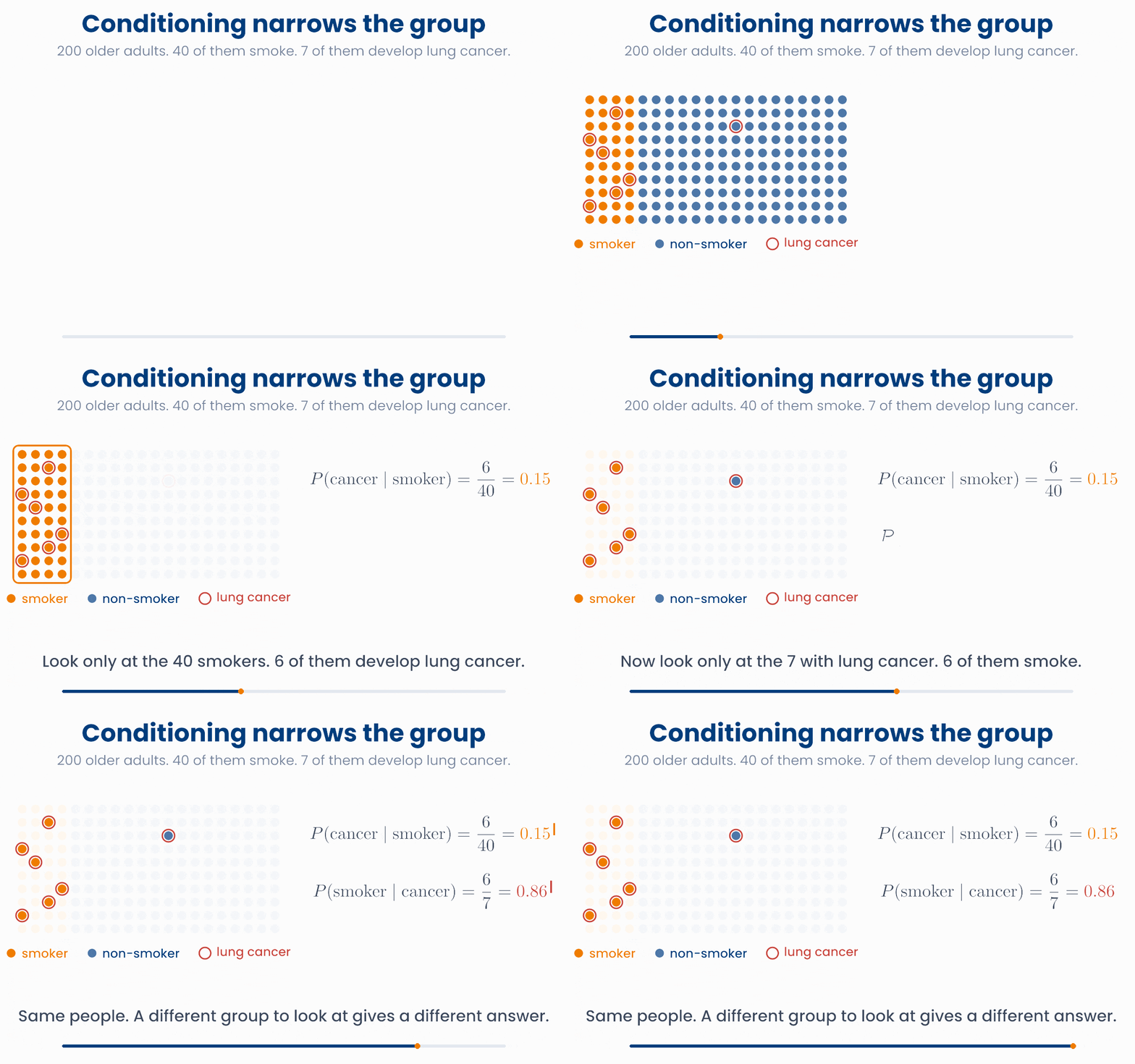
The vertical bar \(\mid\) is read "given". It means: look only at the group named after the bar.
- \(P(\text{cancer} \mid \text{smoker}) = 6/40 = 0.15\). Among the 40 smokers, 6 develop lung cancer.
- \(P(\text{smoker} \mid \text{cancer}) = 6/7 \approx 0.86\). Among the 7 people with lung cancer, 6 smoke.
It is the same people and the same 6 smokers with cancer. The only change is the group you divide by: 40 smokers, or 7 people with cancer. That is why the two answers are so different. Always ask: which group is after the bar?
Conditioning means: look only at one group
Choose a group to look at, and what to count inside it. Orange = smoker, blue = non-smoker, red ring = lung cancer. People outside the group fade.
Conditioning keeps only the people in group \(B\). You count those who also have \(A\), and divide by the size of group \(B\). If you divide both counts by the total number of people, you get the formula:
Check the formula with the smokers
- \(P(\text{cancer and smoker}) = 6/200 = 0.03\).
- \(P(\text{smoker}) = 40/200 = 0.20\).
- \(P(\text{cancer} \mid \text{smoker}) = 0.03 / 0.20 = 0.15\). This is the same as \(6/40\).
Swapping the condition
import numpy as np
smoker = np.zeros(200, dtype=int)
smoker[:40] = 1                     # 40 smokers
cancer = np.zeros(200, dtype=int)
cancer[:6] = 1; cancer[40] = 1      # 6 smokers and 1 non-smoker

print(cancer[smoker == 1].mean())   # 0.15   P(cancer | smoker)
print(smoker[cancer == 1].mean())   # 0.857  P(smoker | cancer)
both = (cancer == 1) & (smoker == 1)
print(both.mean() / smoker.mean()) # 0.15 P(cancer and smoker) / P(smoker)A hospital has 1000 admissions in a year and 50 deaths. 80 of the admitted patients had sepsis, and 20 of those 80 died. What is \(P(\text{death} \mid \text{sepsis})\)?
4 Independence
Does knowing one thing about a patient change the chance of another? If it does, the two events are dependent. If it does not, they are independent.
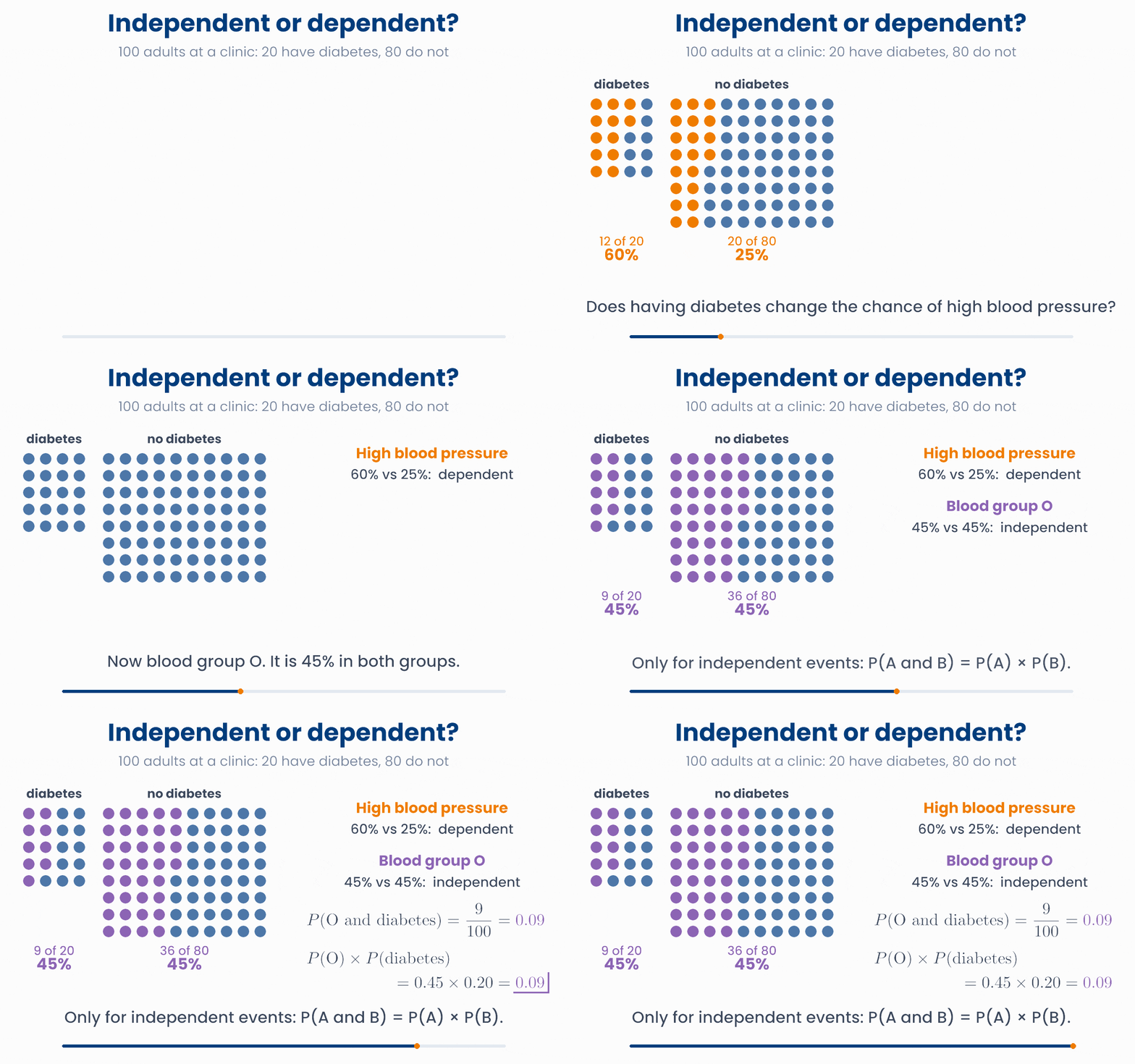
In the animation, 60% of the adults with diabetes have high blood pressure, but only 25% of those without diabetes do. Knowing that someone has diabetes raises the chance. So diabetes and high blood pressure are dependent. This is expected: they share causes such as obesity and age.
Blood group O is 45% in both groups. Knowing about diabetes tells you nothing about blood group. These two events are independent:
Only then can you find the chance of both events by multiplying. Put \(P(A \mid B) = P(A)\) into the formula from section 3 and you get the multiplication rule:
Check it with the animation. \(P(\text{O and diabetes}) = 9/100 = 0.09\), and \(P(\text{O}) \times P(\text{diabetes}) = 0.45 \times 0.20 = 0.09\). They agree. For high blood pressure they do not. \(P(\text{high BP and diabetes}) = 12/100 = 0.12\), but \(P(\text{high BP}) \times P(\text{diabetes}) = 0.32 \times 0.20 = 0.064\). Multiplying dependent events gave about half of the true answer.
Independent means the same chance in every group
Each column is one group of adults; its width is the share of adults in that group. The orange part is the fraction with high blood pressure. Change the sliders, or press "Make them independent".
You used the multiplication rule in Unit 1, for a panel of tests that do not affect each other. In practice, results from different, unrelated patients are usually treated as independent. Two measurements from the same patient, or from members of the same family, usually are not.
Why you will care later
import numpy as np
p_d = 0.20                         # P(diabetes)
p_ht_d, p_ht_nod = 0.60, 0.25      # P(high BP | diabetes), P(high BP | no diabetes)
p_ht = p_d * p_ht_d + (1 - p_d) * p_ht_nod
print(p_ht)              # 0.32   P(high BP)
print(p_d * p_ht_d)      # 0.12   P(high BP and diabetes), the true value
print(p_ht * p_d) # 0.064 what multiplying would give: wrong hereIn a cohort, 30% of all patients are readmitted within 30 days. Among patients who live alone, 30% are also readmitted. What does this suggest?
5 Diagnostic tests
A diagnostic or screening test sorts people into test positive (+) and test negative (−). It can make two kinds of mistake. A false positive is a healthy person who tests positive. A false negative is a person with the disease who tests negative.
Three numbers describe a test and the people it is used on. Each is a probability you can already read:
| Name | As a probability | In words |
|---|---|---|
| Prevalence | \(P(\text{disease})\) | The fraction of the people tested who have the disease. |
| Sensitivity | \(P(+ \mid \text{disease})\) | Among people with the disease, the fraction the test finds. |
| Specificity | \(P(- \mid \text{no disease})\) | Among people without the disease, the fraction the test clears. |
The easiest way to use them is to picture 1000 people and split them twice: first by the truth, then by the test result.
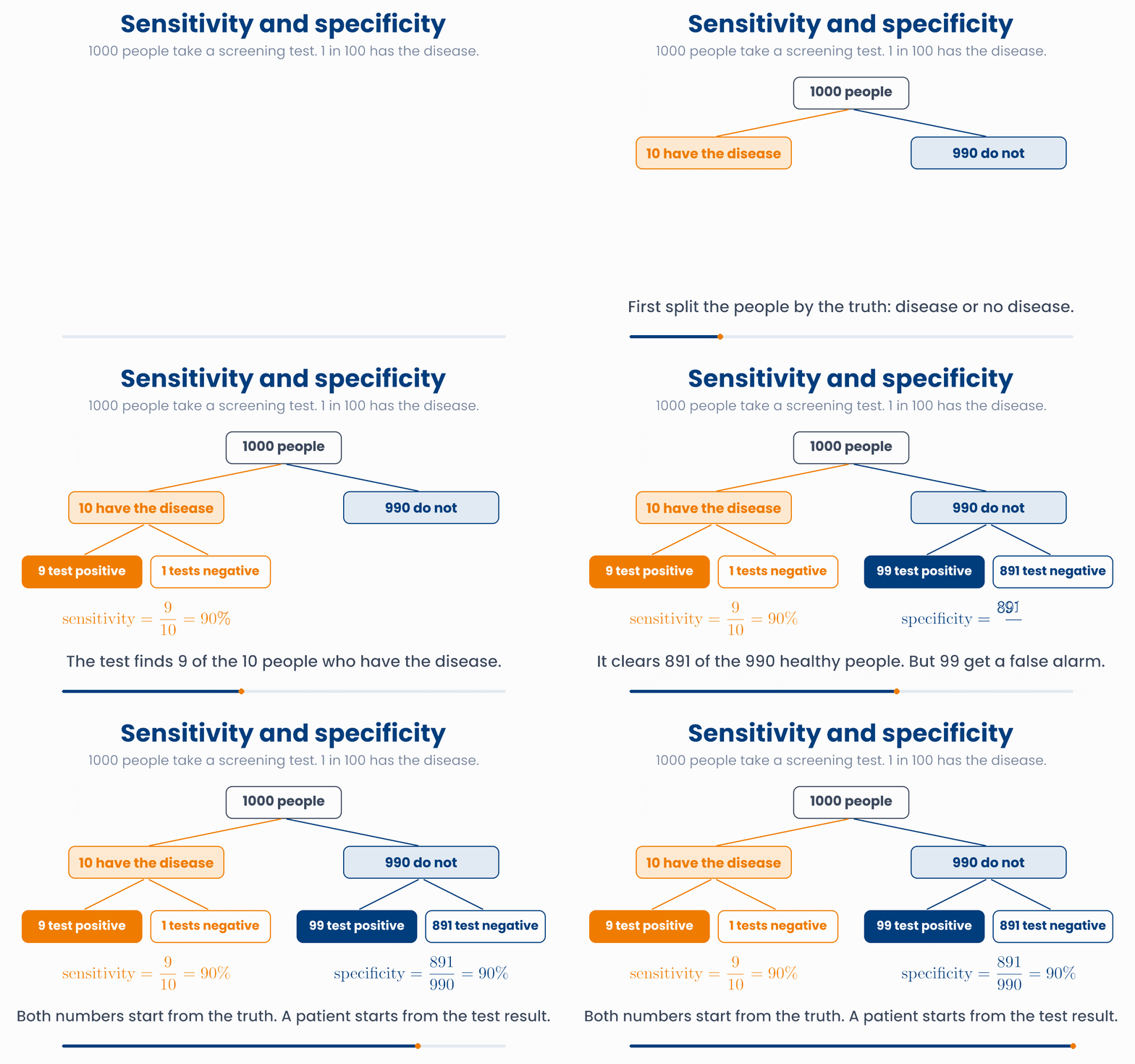
Put the four groups into a 2×2 table. The columns are the truth. The rows are the test result.
| Disease | No disease | Total | |
|---|---|---|---|
| Test + | 9 true positives (TP) | 99 false positives (FP) | 108 |
| Test − | 1 false negative (FN) | 891 true negatives (TN) | 892 |
| Total | 10 | 990 | 1000 |
Sensitivity and specificity are read down the columns:
Many tests give a number, not a yes or a no: a blood level or a risk score. Someone chooses a cut-off. A result above the cut-off counts as positive. Moving the cut-off trades one kind of mistake for the other.
Moving the cut-off trades sensitivity for specificity
Drag on the plot, or use the slider, to move the cut-off. Results to the right of it count as positive. The orange shading is the share of people with the disease that the test finds; the blue shading is the share of healthy people it clears.
A low cut-off misses few people with the disease (high sensitivity) but gives many false alarms (low specificity). A high cut-off does the opposite. No cut-off makes both mistakes vanish, because the two groups overlap.
Why you will care later
import numpy as np
# rows: test +, test -      columns: disease, no disease
table = np.array([[9, 99],
                  [1, 891]])
print(table.sum(axis=0))            # [ 10 990]  people with and without the disease
sens = table[0, 0] / table[:, 0].sum()
spec = table[1, 1] / table[:, 1].sum()
print(sens, spec) # 0.9 0.9A test for a heart condition has a specificity of 95%. What does this mean?
6 Bayes' theorem
Sensitivity tells you \(P(+ \mid \text{disease})\). But a patient with a positive result wants to know the reverse: \(P(\text{disease} \mid +)\). Section 3 showed that swapping the condition can give a very different number. Here is how to get it right.
With counts first. Go back to the 1000 people. 108 of them test positive. Only 9 of those 108 have the disease. So for a person with a positive test:
This number is called the positive predictive value (PPV). The woman in the introduction has about an 8% chance of having the disease, not 90%. This is because the disease is rare. The 990 healthy people are so many that even 10% of them, 99 false alarms, far outnumber the 9 real cases.
The negative predictive value (NPV) is the same idea for a negative result: \(P(\text{no disease} \mid -) = 891/892 \approx 0.999\). A negative screening result is very reassuring.
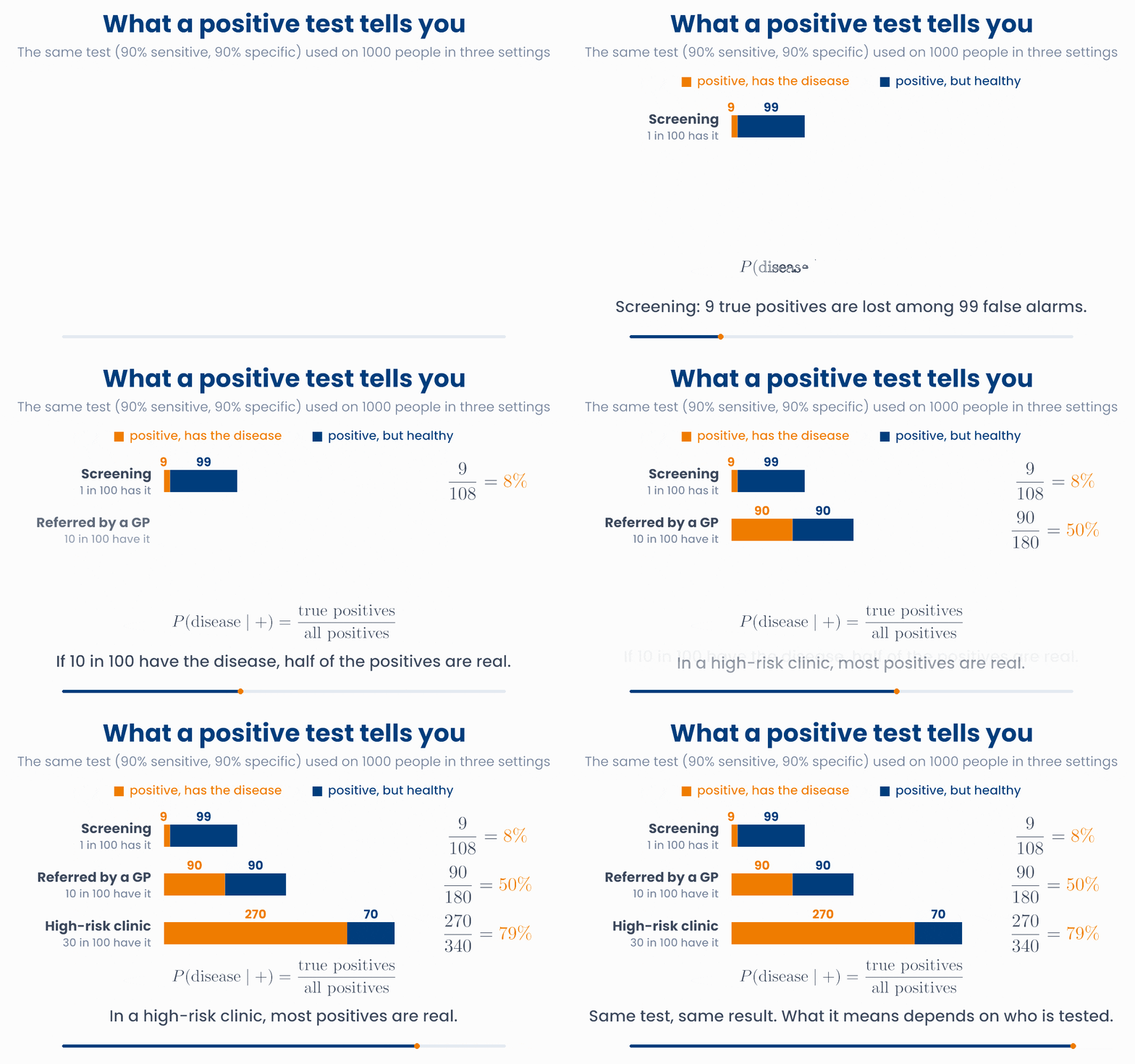
Now use the same test in a high-risk clinic, where 30 in 100 patients have the disease. The PPV is 79%. The test has not changed. The people tested have. The PPV depends on the prevalence.
1000 people, one test: what does a positive result mean?
Change the prevalence, sensitivity and specificity, or press a setting. Tick the box to keep only the people who test positive: the PPV is the orange share of what is left.
Then the formula. Write the counts as probabilities and you get Bayes' theorem. In general it turns \(P(B \mid A)\) into \(P(A \mid B)\):
For a test, \(A\) is "has the disease", written \(D\) to keep it short, and \(B\) is "positive result":
Every piece is something you know. \(P(+ \mid \text{disease})\) is the sensitivity. \(P(\text{disease})\) is the prevalence. \(P(+ \mid \text{no disease}) = 1 - \text{specificity}\) is the false positive rate. \(P(+)\) is the chance of a positive result for anyone: the true positives plus the false positives.
Bayes' theorem for the screening example
- Top: sensitivity × prevalence \(= 0.90 \times 0.01 = 0.009\). These are the 9 true positives in 1000.
- False positives: \((1 - 0.90) \times 0.99 = 0.099\). These are the 99 false positives in 1000. So \(P(+) = 0.009 + 0.099 = 0.108\).
- \(P(\text{disease} \mid +) = 0.009 / (0.009 + 0.099) = 0.009 / 0.108 \approx 0.083\).
Bayes' theorem is a rule for updating what you believe when new evidence arrives:
- The prior is the probability before the evidence. Here it is the prevalence, 1%, also called the pre-test probability.
- The evidence is the test result.
- The posterior is the probability after the evidence. Here it is 8.3%, the post-test probability.
The posterior can become the prior for the next piece of evidence. Suppose the woman takes a second, independent test of the same quality, and it is also positive. Her chance rises from 8.3% to 45%. This is why a positive screening result is followed by a confirmatory test, not by treatment.
Why you will care later
import numpy as np
prev = np.array([0.01, 0.10, 0.30])     # screening, GP referral, high-risk clinic
sens, spec = 0.90, 0.90

ppv = sens * prev / (sens * prev + (1 - spec) * (1 - prev))
print(ppv.round(3))      # [0.083 0.5   0.794]

npv = spec * (1 - prev) / (spec * (1 - prev) + (1 - sens) * prev)
print(npv.round(3)) # [0.999 0.988 0.955]A test has a sensitivity of 80% and a specificity of 96%. It is used on 1000 people, and 50 of them have the disease. About what fraction of the people who test positive have the disease?
7 Check your understanding
Five short questions on this lesson. Nothing is graded or saved outside this browser. If you choose a wrong option you get a hint, and you can try again.
In a surgical ward, 8% of patients develop a wound infection. What is the probability that a patient does not develop one?
A news report says: "90% of people with lung cancer were smokers." Which probability is this?
A gene variant is carried by 20% of people, and 10% of people have a certain blood group. If the two are independent, what fraction of people have both?
Which statement about sensitivity is correct?
A screening test is 95% sensitive and 95% specific. In the screened population, 2% have the disease. Out of 1000 people, about how many of the positives truly have the disease?