

1 Introduction
In lesson 3.1 every curve had one input: time. Real models have many inputs. A risk score for heart disease uses age, blood pressure, cholesterol and smoking. A neural network that reads a chest X-ray has millions of weights. To understand such a model, we ask how its output changes when we change one input. That is a partial derivative. Put all of them together and you get the gradient: the arrow that tells a model how to learn.
Sometimes we need the opposite of a rate: a total. An infusion pump gives 50 mg per hour for 2 hours, then 100 mg per hour for 2 more hours. How much drug went in? Rate times time, added up: \(50 \times 2 + 100 \times 2 = 300\) mg. On a graph of the rate, this total is the area under the line.
A total is an area under a rate
Change the two pump rates. Each shaded block is rate × time, so the total amount of drug given is the shaded area.
When the rate changes all the time, as a drug level does after a tablet, the area under a curve needs the second half of calculus: the integral. It also turns out that every probability for a measurement such as blood pressure is an area under a curve.
What you will be able to do
- Read \(\frac{\partial f}{\partial x}\) and say what it means to change one input and hold the others fixed.
- Say which way the gradient points, and why a model steps the other way.
- Multiply rates along a chain, and know that this is how neural networks learn.
- Read \(\int_a^b f(x)\,dx\) as an area: a total drug exposure, or a probability.
import numpy as np
rate = np.array([50, 50, 100, 100])   # mg per hour, in each of 4 hours
print(np.sum(rate * 1)) # 300 mg: rate x 1 hour, added up2 Partial derivatives
Two blood-pressure drugs, A and B, are given together. The fall in systolic blood pressure, \(R\) (in mmHg), depends on both doses: \(a\) mg of drug A and \(b\) mg of drug B. A function of two inputs, \(R(a, b)\), cannot be drawn as one curve. Instead, we draw a contour map, like a hiking map: each line joins the dose pairs that give the same response.
Now ask: if I give a little more of drug A, and keep drug B the same, how much more does the blood pressure fall? That is a slope in one direction only. It is called a partial derivative:
- \(\frac{\partial R}{\partial a}\): change the dose of A only. Hold the dose of B fixed.
- \(\frac{\partial R}{\partial b}\): change the dose of B only. Hold the dose of A fixed.
Each partial derivative is an ordinary slope from lesson 3.1. You walk across the map along a straight line in one direction, and measure how steeply the function rises. The animation does this for a model's loss \(L\), which depends on two weights, \(w_1\) and \(w_2\).
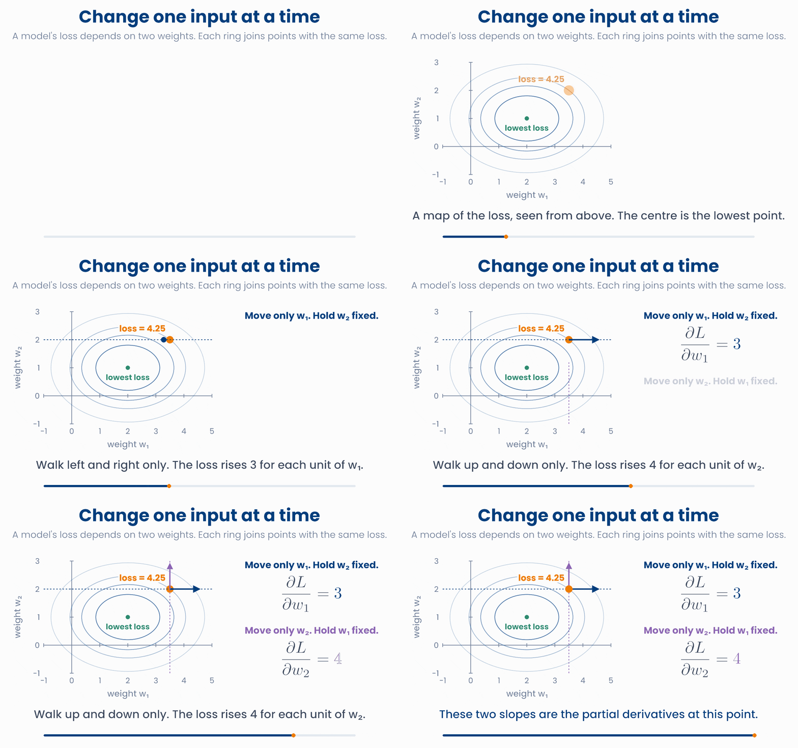
Change one dose, hold the other fixed
Drag the point on the map, or use the sliders. Choose which dose to walk along: the lower plot shows the response along that dashed line only, with its slope. Each map line joins dose pairs with the same fall in blood pressure (in mmHg). The model is made up for teaching.
Notice that the slope for drug A changes a little when you change the dose of drug B. In this made-up model, drug B makes drug A work slightly better. So "how much does one more mg of A help?" has a different answer at different doses of B. This is why a partial derivative always comes with the words "at this point, holding the others fixed".
Why you will care later
def R(a, b):   # fall in BP (mmHg) for a mg of drug A and b mg of drug B
    return 18 * a / (a + 40) + 12 * b / (b + 6) + 0.004 * a * b

h = 1e-6                                           # a tiny step
print(round(R(50, 10), 1))                         # 19.5  mmHg
print(round((R(50 + h, 10) - R(50, 10)) / h, 3))   # 0.129  dR/da
print(round((R(50, 10 + h) - R(50, 10)) / h, 3)) # 0.481 dR/dbA risk model uses age and systolic blood pressure (SBP). For one patient, \(\dfrac{\partial\,\text{risk}}{\partial\,\text{SBP}} = 0.002\) per mmHg. What does this mean?
3 The gradient
A function of two inputs has two partial derivatives at each point. Stack them into a vector, as in Unit 2, and you get the gradient:
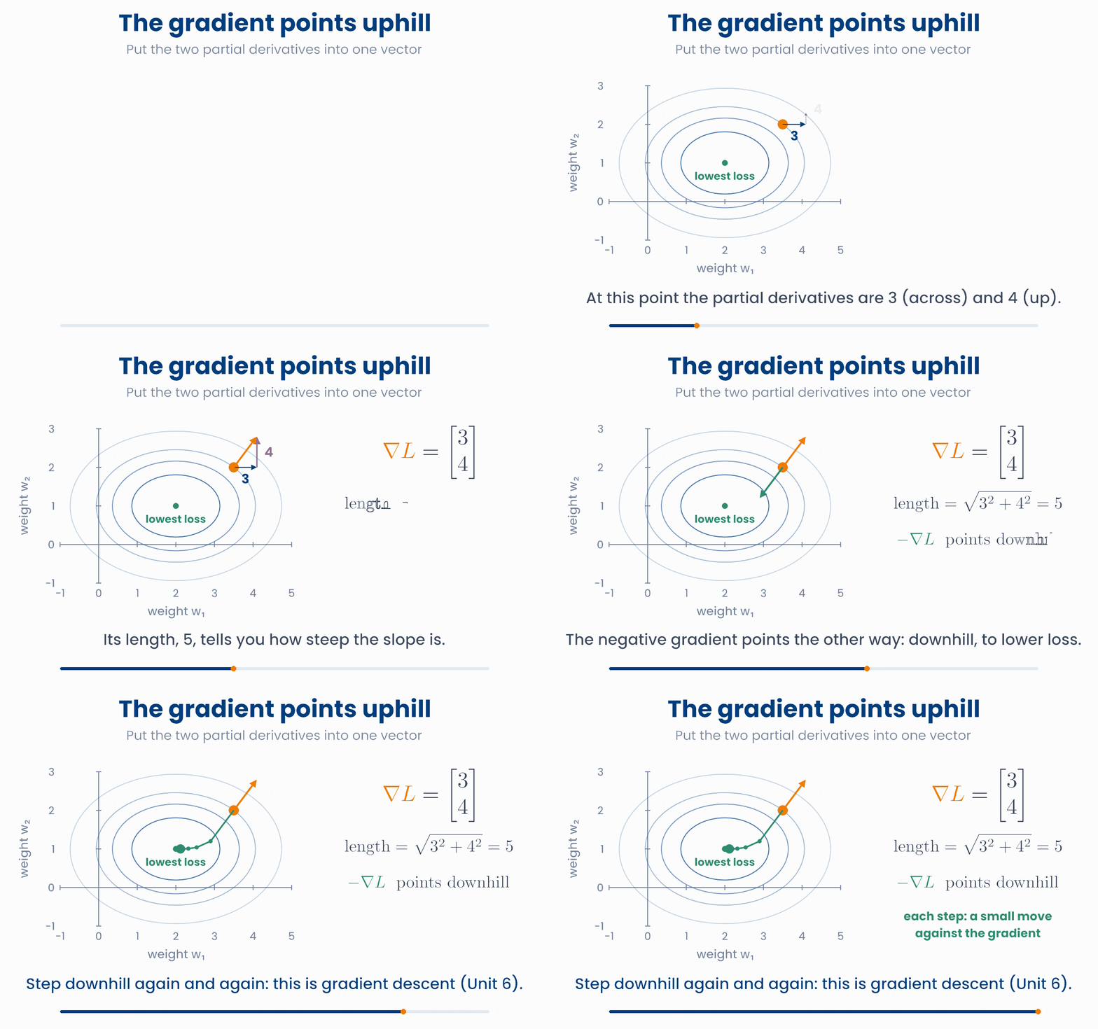
The gradient is an arrow on the map. It has three useful properties:
- It points in the direction in which the function rises fastest: straight uphill.
- Its length says how steep the slope is in that direction. At the point in the animation, \(\nabla L = (3, 4)\), and its length is \(\sqrt{3^2 + 4^2} = 5\).
- It crosses the contour lines at a right angle.
The negative gradient, \(-\nabla L\), points the opposite way: straight downhill, towards a lower loss. That is the direction a model wants to move its weights.
The gradient points uphill; step the other way
Drag the orange point anywhere on the loss map. Blue and purple arrows are the two partial derivatives; the orange arrow is the gradient. Then press the step button a few times and watch the point walk downhill to the lowest loss.
Taking small steps downhill, again and again, is called gradient descent:
In the widget each step uses \(\alpha = 0.2\). From the start point, the first step goes from \((3.5, 2)\) to \((3.5 - 0.2 \times 3,\; 2 - 0.2 \times 4) = (2.9, 1.2)\). Near the bottom the gradient gets short, so the steps get small by themselves. Unit 6 covers gradient descent in full: how to choose the step size, and what can go wrong.
Why you will care later
import numpy as np
w = np.array([3.5, 2.0])                            # the two weights now
grad = np.array([2 * (w[0] - 2), 4 * (w[1] - 1)])   # the 2 partials
print(grad)                     # [3. 4.]
print(np.linalg.norm(grad))     # 5.0        how steep: the length
print(w - 0.2 * grad) # [2.9 1.2] one small step downhillAt the current weights, a model's gradient is \(\nabla L = \begin{bmatrix} -2 \\ 6 \end{bmatrix}\). Which way should the two weights move to lower the loss fastest?
4 The chain rule
Many effects happen in steps. A larger dose raises the blood concentration of a drug. A higher concentration lowers the blood pressure. Each step has its own rate:
- \(\frac{dC}{dD}\): how fast the concentration \(C\) rises with the dose \(D\), here 0.2 mg/L per mg;
- \(\frac{dE}{dC}\): how fast the effect \(E\) (the fall in blood pressure) grows with the concentration, here 3 mmHg per mg/L.
How fast does the effect change with the dose? Follow a change along the chain. Give 10 mg more: the concentration rises by \(10 \times 0.2 = 2\) mg/L, and the effect grows by \(2 \times 3 = 6\) mmHg. That is 6 mmHg for 10 mg, or 0.6 mmHg per mg, which is \(3 \times 0.2\).
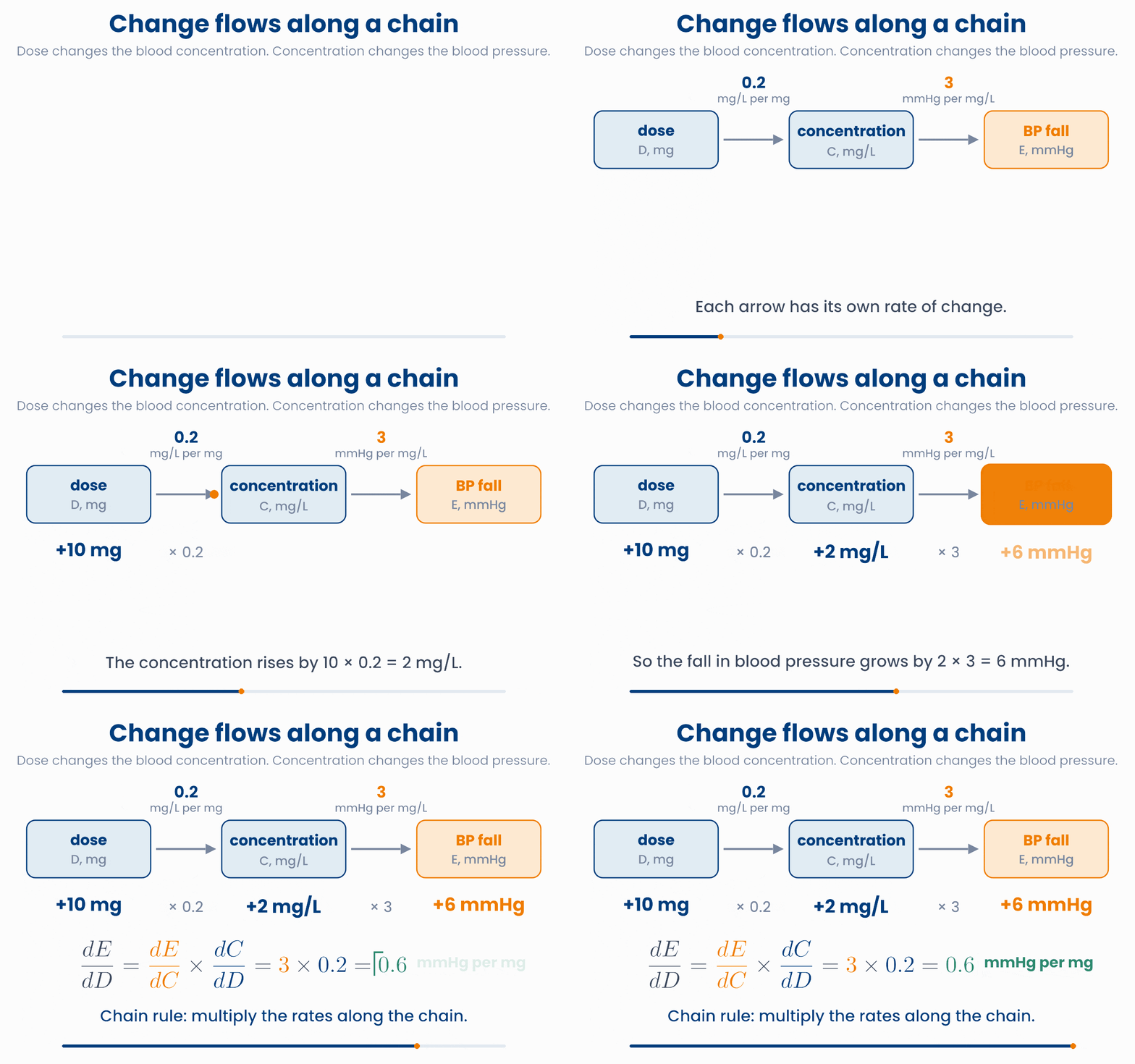
The rule also works when the steps are curves rather than straight lines. Then each rate is the slope at the current point, and the answer holds for small changes around the current dose.
Rates multiply along a chain
Change the rate of each step and the change at the start. Watch the change pass along the chain, and check that the overall rate is the product of the two rates. Switch to the neural network view: it is the same rule.
Why you will care later: this is how neural networks learn
def conc(D):   return 0.2 * D             # mg/L for a dose of D mg
def effect(C): return 30 * C / (C + 4)    # BP fall (mmHg), at most 30

D = 20                                    # mg, so C = 4 mg/L
dC_dD = 0.2                               # mg/L per mg
dE_dC = 30 * 4 / (4 + 4) ** 2             # slope of effect at C = 4: 1.875
print(dE_dC * dC_dD)                      # 0.375  chain rule: mmHg per mg

h = 1e-6                                  # check: nudge the dose a tiny bit
print(round((effect(conc(D + h)) - effect(conc(D))) / h, 3)) # 0.375Each mg of a drug raises its blood concentration by 0.5 mg/L. Each mg/L of concentration lowers the heart rate by 4 beats per minute. How much does each extra mg of the drug lower the heart rate?
5 The integral as an area
After a tablet, how much drug did the patient's body actually see? Not the peak, and not the level at one time, but the total over the whole day. Pharmacologists measure this as the area under the concentration–time curve, the AUC. Generic medicines are judged against the original product by comparing their AUC (together with Cmax). Some cancer drugs, such as carboplatin, are dosed to reach a target AUC.
How do you find the area under a curve? Cut it into thin vertical slices. Each slice is almost a rectangle: its height is the concentration, and its width is a short time \(\Delta t\). Then add up all the rectangles:
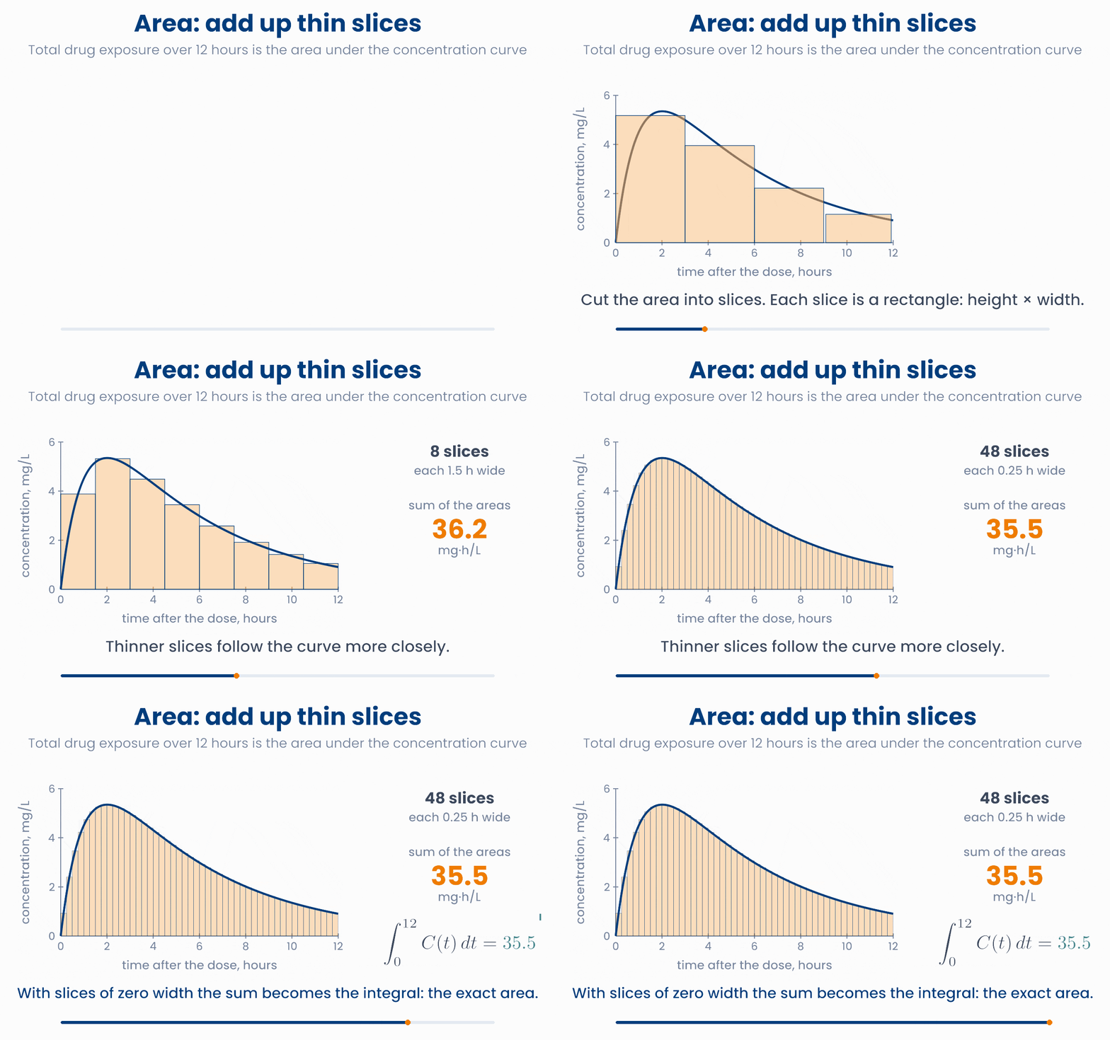
This is called a Riemann sum. With thinner slices the rectangles follow the curve more closely, and the sum gets closer to the true area. When the slices become infinitely thin, the sum becomes the integral:
- The sign \(\int\) is a stretched S, for "sum".
- The numbers at the bottom and the top, 0 and 12, say where to start and where to stop, just as with \(\Sigma\).
- \(dt\) is the width of a very thin slice of time.
- The units are the units of the height times the units of the width: mg/L × hours = mg·h/L.
More slices, closer to the true area
Change the number of slices and where each slice takes its height. Watch the sum of the rectangles approach the exact area, 35.46 mg·h/L.
Derivative and integral undo each other
import numpy as np
t = np.linspace(0, 12, 1201)                 # slices 0.01 hour wide
C = 10 * (np.exp(-0.2 * t) - np.exp(-t))     # mg/L
dt = t[1] - t[0]
auc = np.sum((C[:-1] + C[1:]) / 2 * dt)      # height x width, added up
print(round(auc, 2))                         # 35.46  mg·h/L
# np.trapezoid(C, t) does the same in NumPy 2 (np.trapz in older NumPy)Two tablets of the same drug give the same peak concentration. With tablet B, the level stays near the peak for longer before it falls. Which statement is right?
6 Area as probability
The same idea, "an area is a total", has a second use that you will meet in every statistics course. Systolic blood pressure varies from adult to adult. A density curve shows how the values are spread: it is high where many adults are, and low where few are. Here we use illustrative values: a mean of 125 mmHg and a standard deviation of 15 mmHg.
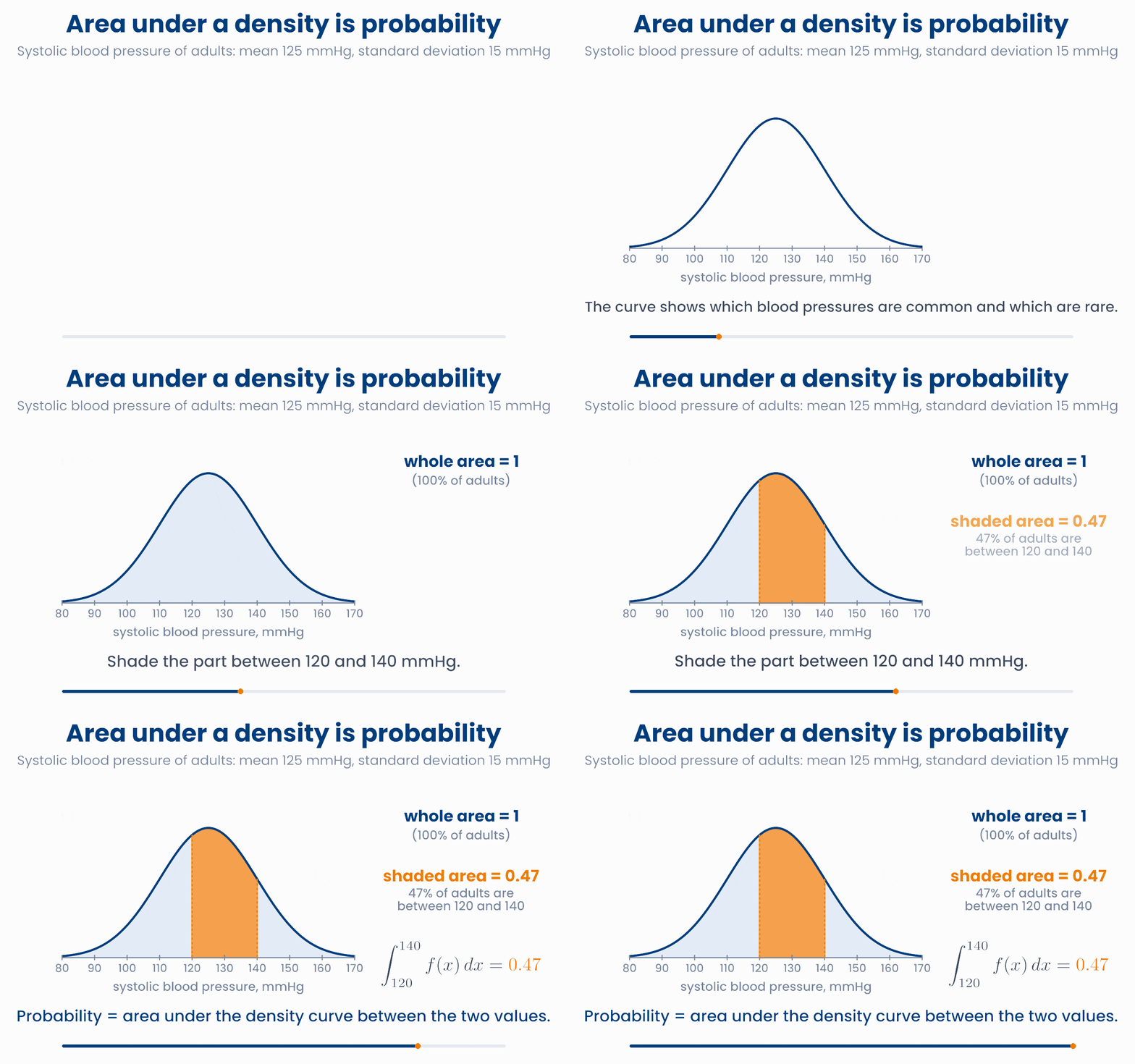
- The area under the curve between two values is the probability that a person's value lies between them. The area between 120 and 140 mmHg is 0.47, so 47% of adults are in that range.
- The total area under the whole curve is 1, because every adult has some blood pressure.
- The height of the curve is not a probability. Only areas are.
Probability is the shaded area
Drag the two orange limits, or use the sliders. The shaded area is the chance that an adult's blood pressure lies between them. The three tiles always add up to 100%.
The ROC AUC is an area too
Why you will care later
import numpy as np
def f(x):                     # density of systolic BP: mean 125, SD 15
    return np.exp(-0.5 * ((x - 125) / 15) ** 2) / (15 * np.sqrt(2 * np.pi))

def area(a, b, n=20000):      # add up thin trapezoid slices from a to b
    x = np.linspace(a, b, n + 1)
    return np.sum((f(x[:-1]) + f(x[1:])) / 2) * (x[1] - x[0])

print(round(area(120, 140), 3))   # 0.472  probability between 120 and 140
print(round(area(25, 225), 3)) # 1.0 the whole areaIn a clinic population, the area under the density curve of HbA1c between 6.5% and 8.0% is 0.18. What does this tell you?
7 Check your understanding
Five short questions on this lesson. Nothing is graded or saved outside this browser. If you choose a wrong option you get a hint, and you can try again.
A model predicts LDL cholesterol (mmol/L) as \(\hat{y} = 1.2 + 0.02 \times \text{age} + 0.05 \times \text{BMI}\). What is \(\dfrac{\partial \hat{y}}{\partial\,\text{BMI}}\)?
At some weights, a loss has gradient \(\nabla L = \begin{bmatrix} 4 \\ -3 \end{bmatrix}\). How steep is it, and which way is downhill?
In a small neural network, the output changes by 3 for each unit change of a hidden value, and the hidden value changes by 0.5 for each unit change of a weight. How fast does the output change with that weight?
A drug level is estimated in the middle of four 2-hour slices: 3, 5, 4 and 2 mg/L. What is the Riemann-sum estimate of the AUC from 0 to 8 hours?
For adult systolic blood pressure, the area under the density between 120 and 140 mmHg is 0.47. What is the probability that an adult is outside this range?