

1 Introduction
A patient takes a tablet. Twice in the next few hours, a blood test shows the same drug level: 4 mg/L. Do the two results mean the same thing?
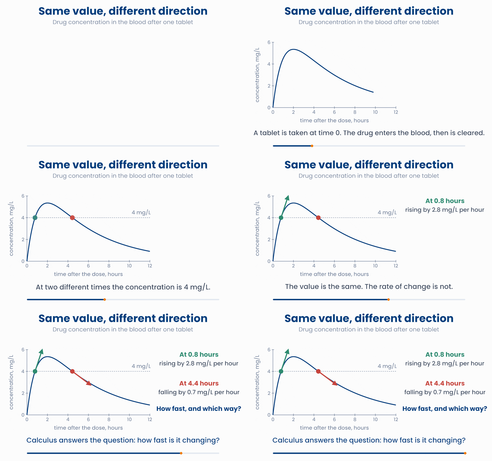
No. At 0.8 hours the drug is still being absorbed, and the level is rising by about 2.8 mg/L every hour. At 4.4 hours the body is clearing the drug, and the level is falling by about 0.7 mg/L every hour. The value tells you where the patient is now. The rate of change tells you where they are going next.
Questions about rates come up all the time in medicine:
- Drug levels. How fast does the concentration rise after a dose, and how fast is the drug cleared? (mg/L per hour)
- Tumour growth. How fast is a tumour growing between two scans? (cm³ per month)
- Heart rate. How fast does it climb at the start of exercise, and how fast does it recover afterwards? (beats per minute, per minute)
The mathematics of change is called calculus. It has two halves. The derivative measures how fast something is changing. That is this lesson. The integral adds up a total, such as the total amount of drug a patient was exposed to. That is the next lesson.
What you will be able to do
- Work out an average rate of change and give it the right units.
- Read \(\frac{dy}{dx}\) and \(f'(x)\) aloud, and say what a derivative tells you about a curve.
- Find a peak, or the best model, by looking for the place where the slope is zero.
With measurements taken at regular times, the simplest look at change is the difference from one measurement to the next. NumPy does this with np.diff:
import numpy as np
hr = np.array([72, 95, 118, 132, 140, 144])  # beats/min, once a minute
print(np.diff(hr))   # [23 23 14  8  4]  the change in each minute
The heart rate climbs fast at first (23 beats per minute, each minute), then more and more slowly as it levels off.
2 Average rate of change
Start with the simplest question. A patient's drug level is 4.31 mg/L at 4 hours after the tablet, and 2.02 mg/L at 8 hours. On average, how fast did it fall between these two times?
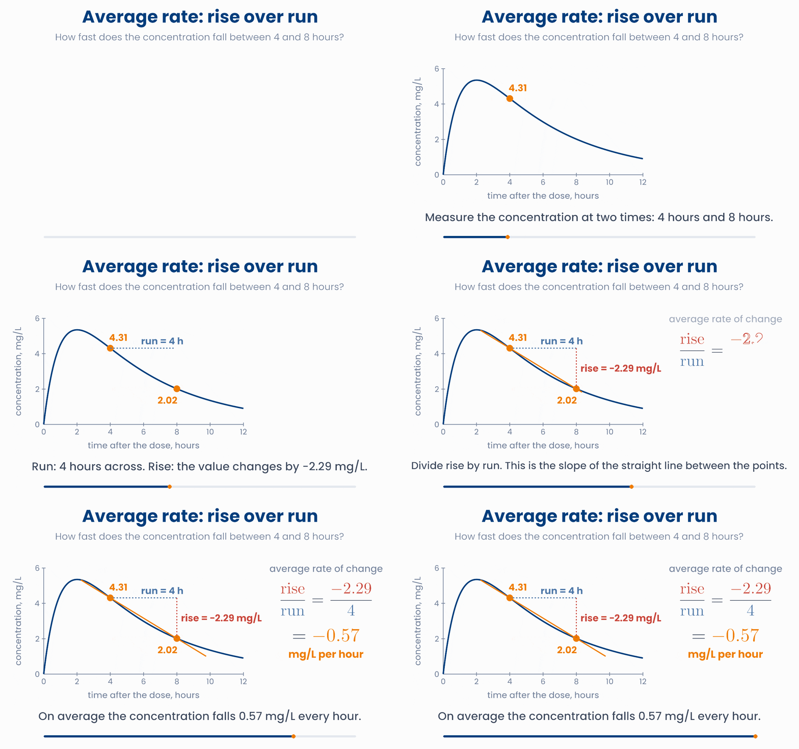
Divide the change in concentration by the change in time:
- The average rate of change is the change in the output divided by the change in the input: "rise over run". It is the slope \(m\) of lesson 1.2, for the straight line that joins the two points.
- A straight line that joins two points on a curve is called a secant line.
- The sign gives the direction. Here the rate is negative, so the level is falling.
- The units are the units of the output per unit of the input. Concentration is in mg/L and time is in hours, so the rate is in mg/L per hour.
Rise over run between two blood tests
Drag either point along the curve, or use the sliders. Watch the sign of the average rate: positive while the drug is absorbed, negative while it is cleared.
An average can hide what happened
import numpy as np
def C(t):                                 # mg/L, t hours after the tablet
    return 10 * (np.exp(-0.2 * t) - np.exp(-t))

print(round(C(4), 2), round(C(8), 2))     # 4.31 2.02
rate = (C(8) - C(4)) / (8 - 4)            # rise over run
print(round(rate, 2)) # -0.57 mg/L per hourA tumour has a volume of 2.0 cm³ at diagnosis and 3.5 cm³ six months later. What is its average rate of growth?
3 The derivative: the rate at one moment
An average over 4 hours is useful. But a doctor may want to know how fast the level is changing right now, at one moment. At a single moment there is no gap: the run is 0, and "rise over run" would be \(0/0\), which has no meaning.
The way out is to make the gap small, then smaller still, and watch what happens to the average rate. Take the moment \(t = 1\) hour after the tablet, and a gap of \(h\) hours:
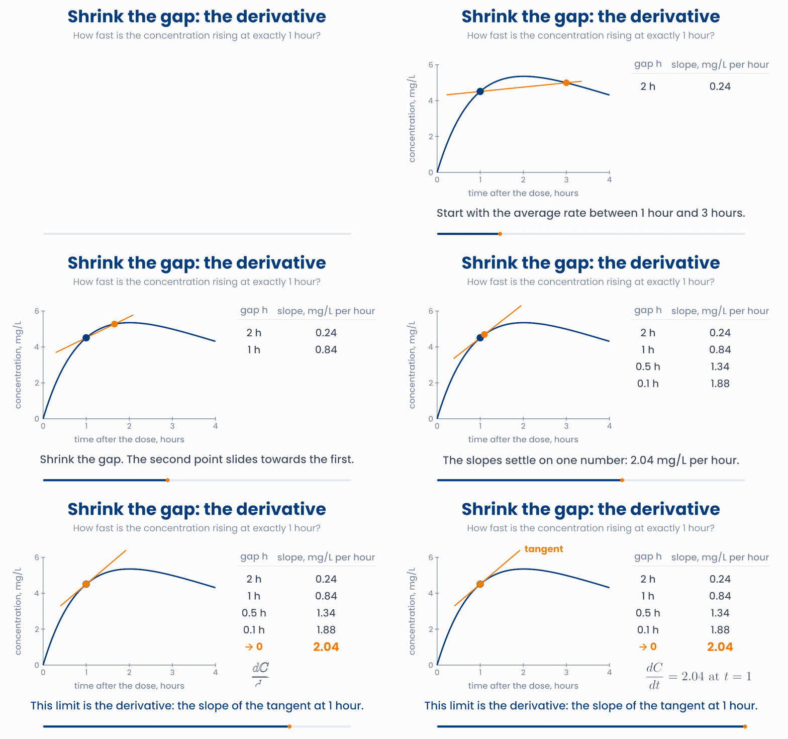
| Gap \(h\) | Average rate from 1 hour to \(1 + h\) hours |
|---|---|
| 2 hours | 0.24 mg/L per hour |
| 1 hour | 0.84 mg/L per hour |
| 0.5 hour | 1.34 mg/L per hour |
| 0.1 hour | 1.88 mg/L per hour |
| 0.01 hour | 2.02 mg/L per hour |
| closer and closer to 0 | 2.04 mg/L per hour |
As the gap shrinks, the average rates settle on one number: 2.04 mg/L per hour. This number is the derivative, the rate of change at one moment. In the picture, the secant line turns into the tangent line. The tangent touches the curve at one point and runs in the same direction as the curve there. The derivative is the slope of the tangent.
The word limit, \(\lim\), means "the value this settles on as \(h\) gets closer and closer to 0". You will not need to work out limits by hand. You only need the idea: a derivative is rise over run, with a very, very small run.
Papers write the derivative in two ways. You will meet both:
| Symbol | Say it as | What it means |
|---|---|---|
| \(\Delta y\) | delta y | The change in \(y\) between two points. |
| \(\dfrac{dy}{dx}\) | d y by d x | The derivative: how fast \(y\) changes as \(x\) changes. |
| \(f'(x)\) | f prime of x | The derivative of the function \(f\), at the input \(x\). |
| \(\dfrac{dC}{dt}\) | d C by d t | How fast the concentration \(C\) changes with time \(t\). |
Common mistake
Shrink the gap until the secant becomes the tangent
Make the gap h smaller and smaller. Watch the orange secant line turn into the dashed tangent, and the average rate settle on the derivative. Then try other times t.
Why you will care later
import numpy as np
def C(t):
    return 10 * (np.exp(-0.2 * t) - np.exp(-t))

for h in [1, 0.1, 0.01, 0.001]:              # shrink the gap
    print(h, round((C(1 + h) - C(1)) / h, 3))
# 1 0.841 0.1 1.88 0.01 2.025 0.001 2.04 it settles on 2.04A paper reports \(\dfrac{dV}{dt} = 0.4\) cm³ per month for a tumour at month 6, where \(V\) is the volume and \(t\) is the time. What does this say?
4 Reading a derivative
The sign and the size of a derivative tell you the shape of the curve at that point:
| Derivative | The curve is | After a tablet |
|---|---|---|
| positive, \(f'(x) > 0\) | rising | the drug is being absorbed |
| negative, \(f'(x) < 0\) | falling | the drug is being cleared |
| zero, \(f'(x) = 0\) | flat, for a moment | the level is at its peak |
| far from 0 | steep | the level changes fast |
| close to 0 | nearly flat | the level changes slowly |
Every point on a curve has its own slope. So we can work out the slope at every time and draw all of these slopes as a second curve. This new curve is the derivative \(f'\). It is a function in its own right.
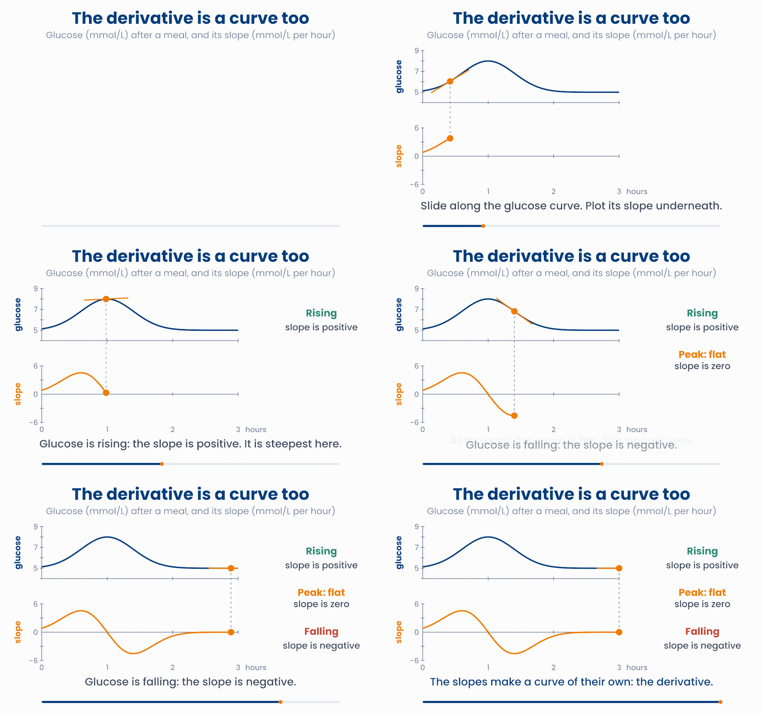
The drug after a tablet behaves in the same way. In the absorption phase the slope is positive: the drug enters the blood faster than the body clears it. At the peak, about 2 hours after the tablet, the slope is zero. In the elimination phase the slope is negative. It is most negative at about 4 hours, then moves back towards zero as less and less drug is left.
A curve and its derivative, side by side
Drag along either plot, or use the slider. The top plot shows the concentration and its tangent. The bottom plot shows the slope of that tangent. Find the time where the slope crosses zero.
import numpy as np
t = np.linspace(0, 12, 1201)              # every 0.01 hour
C = 10 * (np.exp(-0.2 * t) - np.exp(-t))
slope = np.gradient(C, t)                 # the slope at every time
# the slopes at 1, 2 and 4 hours:
print(np.round(slope[[100, 200, 400]], 2))   # [ 2.04  0.01 -0.72]
print(t[slope < 0][0]) # 2.02 first time the slope is negativeAfter a meal, the slope of a patient's glucose curve is positive before 1 hour, zero at 1 hour, and negative after 1 hour. What happened at 1 hour?
5 A few derivatives worth knowing
Nobody works out derivatives by hand in applied work: software does it for you. But a few results are worth knowing by sight, because they explain how drugs, tumours and models behave.
| Function | Derivative | What it says |
|---|---|---|
| \(c\) | \(0\) | A constant does not change, so its rate of change is 0. |
| \(mx + c\) | \(m\) | A straight line has the same slope everywhere: its slope \(m\). |
| \(x^2\) | \(2x\) | The further from 0, the steeper the curve. |
| \(e^x\) | \(e^x\) | The slope always equals the height. This is what makes \(e\) special. |
| \(C = C_0 e^{-kt}\) | \(-kC\) | Exponential decay: the slope is \(-k\) times the curve itself. The rate is proportional to the amount that is left. |
| \(\sigma(z)\) | \(\sigma(1 - \sigma)\) | The sigmoid is steepest in the middle, at \(z = 0\), where its slope is \(0.5 \times 0.5\), or 0.25. |
Two more facts let software build any other derivative from these. Multiplying a function by a number multiplies its slope by the same number. The slope of a sum is the sum of the slopes. For example, the slope of \(3x^2 + 5\) is \(3 \times 2x + 0 = 6x\).
Check the table: a curve and its slope
Choose a function from the table, then move x. The blue curve is f(x) with its tangent. The orange dashed curve is the derivative: its height at each x is the slope of the blue curve there.
The fifth row deserves a closer look. In lesson 1.2, a drug cleared by the body followed \(C(t) = C_0 e^{-kt}\). Its derivative gives a very short rule:
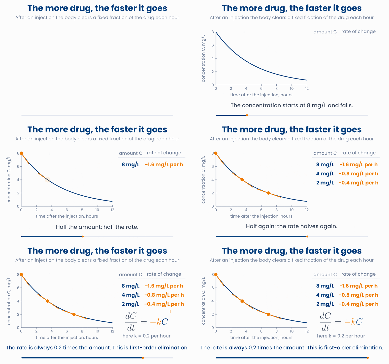
This is first-order elimination, and it describes most drugs at normal doses. The body clears a fixed fraction \(k\) of the drug each hour, so the more drug there is, the faster it goes. With \(k = 0.2\) per hour, a level of 8 mg/L falls by 1.6 mg/L per hour, but a level of 4 mg/L falls by only 0.8 mg/L per hour. As the level gets close to zero, so does the rate. This is why the curve never quite reaches zero.
Growth works the same way with a plus sign. Cells that divide freely follow \(\frac{dN}{dt} = +rN\): the more cells there are, the faster their number grows. This is exponential growth, from lesson 1.2.
First-order elimination: rate = −k × amount
Change the rate constant k and the time t. The orange line is the tangent at time t. Check the third tile: rate divided by concentration is always −k.
Why you will care later
import numpy as np
k = 0.2                              # elimination rate constant, per hour
t = np.array([0, 3.47, 6.93])        # 0, 1 and 2 half-lives, hours
C = 8 * np.exp(-k * t)               # mg/L
print(np.round(C, 1))                # [8. 4. 2.]
print(np.round(-k * C, 1)) # [-1.6 -0.8 -0.4] rate = -kCA drug is cleared by first-order elimination with \(k = 0.1\) per hour. When its concentration is 20 mg/L, how fast is the concentration falling?
6 Maxima and minima
Look again at a curve with a peak. Just before the peak, the curve rises and the slope is positive. Just after, it falls and the slope is negative. At the very top, the slope passes through zero. The same happens at the bottom of a valley, the other way round. So:
This one fact is behind two ideas that you will meet again and again.
Peak concentration. Pharmacologists sum up a concentration curve by its Cmax, the highest concentration, and its tmax, the time when it happens. For our tablet, the slope is zero at about 2.0 hours, and the level there is 5.35 mg/L. So \(t_{\max} \approx 2.0\) h and \(C_{\max} \approx 5.35\) mg/L.
The best model. A model's loss measures how badly its predictions miss the real values. Suppose we must predict the systolic blood pressure of the five patients from lesson 1.1 (128, 141, 119, 135 and 152 mmHg) with one single number \(m\). A common loss is the mean squared error:
The loss curve is a valley. Its lowest point, where \(\frac{dL}{dm} = 0\), is at \(m = 135\) mmHg, which is exactly the mean of the five patients. The best model sits at the bottom of the loss curve.
Find the point where the slope is zero
Choose a curve. Then drag the point, or use the slider, until the slope reads 0. For the drug you are looking for the peak; for the loss you are looking for the bottom.
Zero slope: a peak, a valley, or a pause?
Why you will care later
import numpy as np
t = np.linspace(0, 12, 1201)                 # every 0.01 hour
C = 10 * (np.exp(-0.2 * t) - np.exp(-t))
i = np.argmax(C)
print(round(t[i], 2), round(C[i], 2))        # 2.01 5.35   tmax and Cmax

bp = np.array([128, 141, 119, 135, 152])
m = np.linspace(110, 160, 501)               # candidate predictions
loss = ((bp[:, None] - m) ** 2).mean(axis=0) # mean squared error for each m
print(m[np.argmin(loss)], bp.mean()) # 135.0 135.0 same as the meanAt the current value of a model's weight \(w\), the loss curve has slope \(\dfrac{dL}{dw} = -3\). To make the loss smaller, what should you do?
7 Check your understanding
Five short questions on this lesson. Nothing is graded or saved outside this browser. If you choose a wrong option you get a hint, and you can try again.
During 4 minutes of exercise, a patient's heart rate rises from 70 to 150 beats per minute. What is the average rate of change?
Tumour volume \(V\) is measured in cm³ and time \(t\) in months. What are the units of \(\dfrac{dV}{dt}\)?
A risk model turns a score \(z\) into a probability with the sigmoid, \(\sigma(z)\). Where does a small change in the score change the risk the most?
A drug follows first-order elimination. At 12 mg/L its level falls by 1.2 mg/L per hour. How fast does it fall later, when the level is 6 mg/L?
At \(t_{\max}\), the time of the peak concentration, what is the value of \(\dfrac{dC}{dt}\)?