

1 Introduction
In Lesson 2.1 you computed one patient's risk score with a dot product: multiply each measurement by its weight, then add up. A real study has thousands of patients. You want a prediction for every one of them, from the same weights.
Matrices let you write all of those dot products in one short line:
Read it as: take the data matrix \(X\) (one row per patient), combine every row with the same weights \(\boldsymbol{\beta}\) (the Greek letter beta), and you get a vector \(\hat{\mathbf{y}}\) of predictions ("y hat"). This one line is the heart of linear regression, and it is the first step inside logistic regression and neural networks too.
Matrices do more than predict. A matrix can move every point in a cloud of data at once. It can describe two equations with two unknowns, and its inverse can solve them. And a matrix built from the data can show you the direction in which patients differ most, which is the idea behind principal component analysis (PCA).
What you will be able to do
- Read \(\hat{\mathbf{y}} = X\boldsymbol{\beta}\) and say what it computes for each patient, including the column of 1s.
- Tell from the shapes whether two matrices can be multiplied, and what shape the result has.
- Say what the transpose \(X^{\mathsf{T}}\) and the inverse \(A^{-1}\) do, and when an inverse does not exist.
- Explain PCA in one sentence: it finds the direction of greatest spread.
2 Matrix times vector: a prediction for every patient
A simple model predicts systolic blood pressure from age and BMI:
The 80 is the intercept: a starting value that is added for every patient. The 0.5 says that each extra year of age adds 0.5 mmHg, and the 1 says that each extra unit of BMI adds 1 mmHg. (These are made-up teaching numbers.)
To make every prediction a plain dot product, we add a column of 1s to the data. Then each row reads (1, age, BMI), the weights read \(\boldsymbol{\beta} = (80, 0.5, 1)\), and the intercept is just \(80 \times 1\).
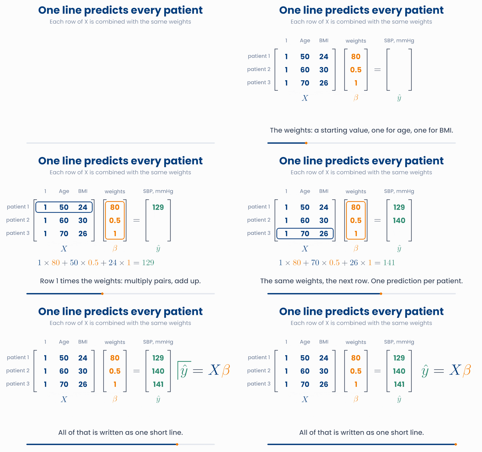
This is the matrix-vector product \(X\boldsymbol{\beta}\). Take each row of \(X\) in turn, do the dot product with \(\boldsymbol{\beta}\), and write the answer in that row of the result.
Each row, the same weights
Move the patient slider down the rows: each row of X is combined with the orange weights β (multiply pairs, add up) to give one prediction. Then change a weight: every prediction changes at once, because every row uses the same weights.
The sizes must fit. \(X\) has \(n\) rows and \(p\) columns, so \(\boldsymbol{\beta}\) must have exactly \(p\) numbers: one weight per column. The result has \(n\) numbers: one prediction per patient.
Why you will care later
import numpy as np
X = np.array([[1, 50, 24],
              [1, 60, 30],
              [1, 70, 26]])       # a column of 1s, age, BMI
beta = np.array([80, 0.5, 1])     # intercept, per year, per BMI unit
print(X @ beta) # [129. 140. 141.] one prediction per patient\(X\) has 100 rows (patients) and 4 columns (a column of 1s, age, BMI, HbA1c). \(\boldsymbol{\beta}\) has 4 numbers. What is \(X\boldsymbol{\beta}\)?
3 Matrix times matrix, and shapes
Suppose you want to compare two models: one set of weights in column 1 of a matrix \(B\), another in column 2. Then \(XB\) is simply \(X\) times each column of \(B\), side by side. You get two predictions for every patient.
Each entry of a matrix product is a dot product: a row of the first matrix with a column of the second. A dot product needs two lists of the same length. That gives the rule for shapes:
Can these two matrices be multiplied?
Change the number of rows and columns of A and B. AB exists only when the columns of A match the rows of B. Watch the result's shape, and check BA too.
Common mistake
A matrix can also be seen as a machine that moves points. Multiply every point of a data cloud by the same 2 × 2 matrix, and the whole cloud is stretched, turned or squashed in one go. This is called a linear transformation.
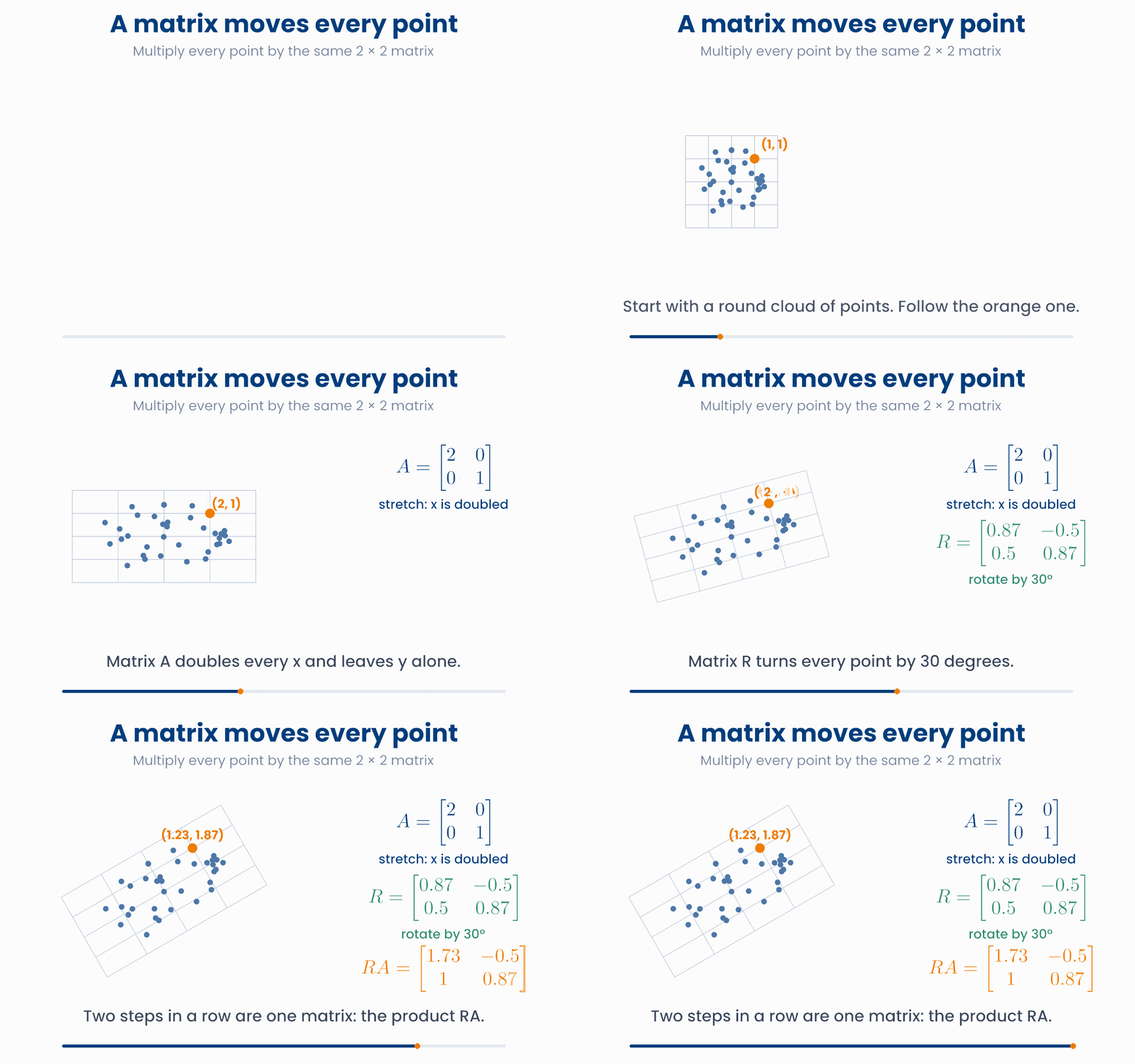
Each column of the matrix tells you where one axis arrow goes. In the stretch matrix \(\begin{bmatrix} 2 & 0 \\ 0 & 1 \end{bmatrix}\), column 1 says that the arrow \((1, 0)\) goes to \((2, 0)\): twice as long. Column 2 says that \((0, 1)\) stays where it is. Doing \(A\) first and then \(R\) is the single matrix \(RA\). (Read it from right to left: \(A\) acts first.)
A 2 × 2 matrix moves the whole cloud
Move the four numbers of the matrix, or press a preset. Grey dots are the original cloud and blue dots are where the matrix sends them. The orange and green arrows are the two columns of the matrix.
Changing units is a transformation too. Converting the second measurement from mmol/L to mg/dL is the matrix \(\begin{bmatrix} 1 & 0 \\ 0 & 18 \end{bmatrix}\): it stretches one axis by 18, exactly the distortion you saw in the distance figure of Lesson 2.1.
import numpy as np
X = np.ones((100, 3))     # 100 patients, 3 columns
B = np.ones((3, 2))       # two sets of weights, one per column
print((X @ B).shape)      # (100, 2)   two predictions per patient

B_bad = np.ones((4, 2))
# X @ B_bad # ValueError: the inner sizes 3 and 4 do not match\(A\) is \(50 \times 3\) and \(B\) is \(3 \times 4\). Which statement is true?
4 The transpose
Sometimes you need a matrix turned on its side. The transpose of \(X\), written \(X^{\mathsf{T}}\) ("X transpose"), swaps rows and columns: row 1 of \(X\) becomes column 1 of \(X^{\mathsf{T}}\), and so on. No number changes. Only its position changes.
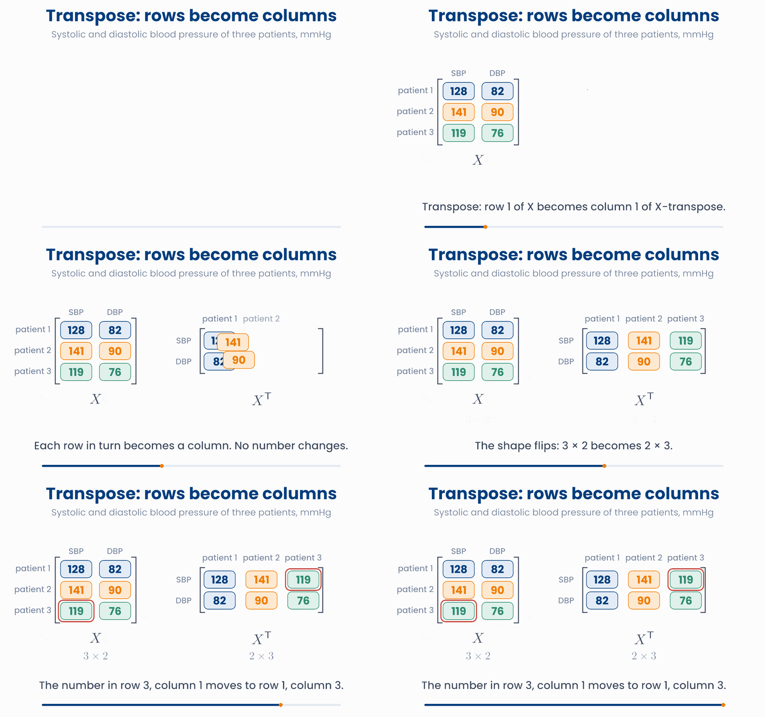
- If \(X\) is \(n \times p\), then \(X^{\mathsf{T}}\) is \(p \times n\).
- The entry in row \(i\), column \(j\) of \(X\) is the entry in row \(j\), column \(i\) of \(X^{\mathsf{T}}\).
- Transposing twice gives back the original: \((X^{\mathsf{T}})^{\mathsf{T}} = X\).
Turn the table on its side
Click any number to follow it, then press Transpose. The selected number is orange; the rest of its patient is blue. A patient's row becomes a column.
You will meet the transpose all the time in formulas. Two common uses:
- One patient's prediction is often written \(\hat{y}_i = \mathbf{x}_i^{\mathsf{T}}\boldsymbol{\beta}\). Here \(\mathbf{x}_i\) is patient \(i\)'s column vector; the transpose lays it down as a row so that it can multiply \(\boldsymbol{\beta}\). It is just the dot product \(\mathbf{x}_i \cdot \boldsymbol{\beta}\).
- \(X^{\mathsf{T}}X\) is \((p \times n)(n \times p) = p \times p\): one number for every pair of features. Each entry adds up, over all patients, the product of two features. When the features are centred (their mean subtracted first), \(X^{\mathsf{T}}X\) divided by \(n - 1\) is the covariance matrix: it summarises how the features move together.
import numpy as np
X = np.array([[128, 82],
              [141, 90],
              [119, 76]])      # 3 patients: SBP, DBP
print(X.shape)        # (3, 2)
print(X.T)            # [[128 141 119]
                      #  [ 82  90  76]]
print(X.T.shape)      # (2, 3)
print((X.T @ X).shape) # (2, 2) one number per pair of features\(X\) has 200 rows (patients) and 5 columns (features). What is the shape of \(X^{\mathsf{T}}X\)?
5 Solving equations with a matrix
A pharmacy needs 500 mL of a 6% glucose solution for a patient. That is 30 g of glucose in 500 mL. It has a 5% stock and a 10% stock. How much of each should it mix?
Call the volumes \(x\) mL (5% stock) and \(y\) mL (10% stock). Two facts must both be true:
This is a system of linear equations: two equations, two unknowns. Each equation on its own is a straight line of possible answers. The solution is the point that lies on both lines: where they cross.
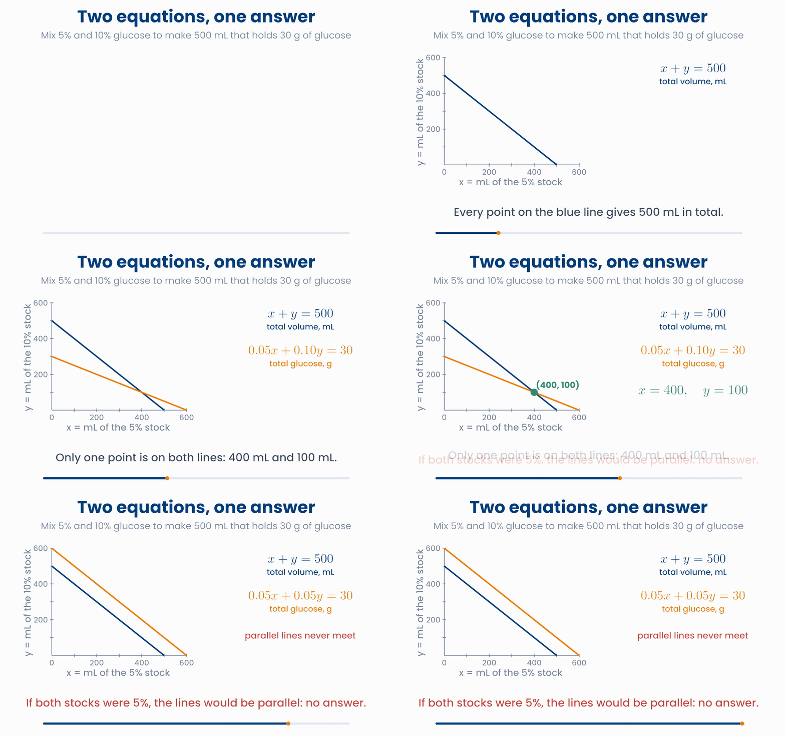
Use 400 mL of the 5% stock and 100 mL of the 10% stock. Check: \(400 + 100 = 500\) mL and \(0.05 \times 400 + 0.10 \times 100 = 20 + 10 = 30\) g.
In matrix form the whole system is one line, \(A\mathbf{x} = \mathbf{b}\):
For one ordinary equation such as \(5x = 20\), you divide: \(x = 20 / 5 = 4\). Matrices have no division. Instead, many square matrices have an inverse, written \(A^{-1}\). The inverse undoes what \(A\) does, so:
You will never need to find an inverse by hand. NumPy does it, and for solving a system it has an even better tool, np.linalg.solve.
The answer is where the lines cross
Change the strength of the second stock and the strength you want to make. The green point is the mix. Set the second stock to 5% and the lines become parallel.
Sometimes there is no unique answer. If both stocks were 5%, the second equation would be \(0.05x + 0.05y = 30\). That says the same thing about the mix as the first equation (it is just 0.05 times it), but with a different total. The lines are parallel. There is no solution, and the matrix \(\begin{bmatrix} 1 & 1 \\ 0.05 & 0.05 \end{bmatrix}\) has no inverse. A matrix without an inverse is called singular.
The same thing happens with data. If two columns of \(X\) carry the same information (body weight in kg and body weight in pounds, or two lab tests that always move together), the model cannot decide how to share the weight between them. Features like this are called collinear. Then \(X^{\mathsf{T}}X\) has no inverse, or nearly none, and the fitted coefficients become unstable.
import numpy as np
A = np.array([[1,    1   ],
              [0.05, 0.10]])     # volume row, glucose row
b = np.array([500, 30])          # 500 mL in total, 30 g of glucose
print(np.linalg.solve(A, b))     # [400. 100.]   mL of 5% stock, mL of 10% stock
print(np.linalg.inv(A) @ b)      # [400. 100.]   the same, with the inverse

A_bad = np.array([[1, 1], [0.05, 0.05]])
# np.linalg.solve(A_bad, b)      # LinAlgError: Singular matrix
Why you will care later
A model includes both body weight in kg and the same body weight in pounds as two features. Why is this a problem?
6 Eigenvectors and PCA
Systolic and diastolic blood pressure move together: patients with a high systolic pressure usually have a high diastolic pressure too. On a plot, the patients form a long, thin cloud that runs diagonally.
Now ask: in which direction do the patients differ most? Draw a line through the middle of the cloud and drop every patient onto it. The spread (variance) of those dropped points depends on the direction of the line. Along the long axis of the cloud the spread is largest. That direction is the first principal component, PC1. The second, PC2, is at a right angle to it and carries what is left.
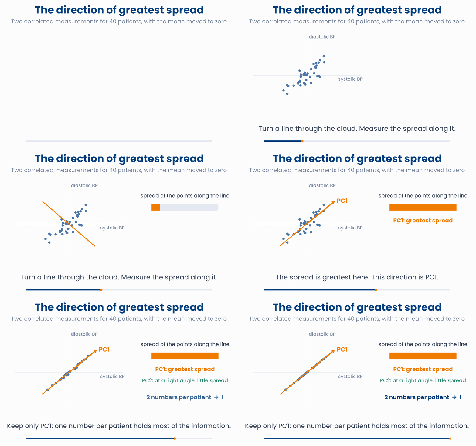
Find the direction of greatest spread
Turn the line with the slider. The orange marks are the patients dropped onto the line, and the lower plot shows their variance for every angle. Find the peak, or press the button. Tick the box to test whether the direction is an eigenvector.
Where do eigenvectors come in? Put the variances and the covariance of the two measurements into a 2 × 2 matrix, the covariance matrix \(C\). Multiply a direction \(\mathbf{v}\) by \(C\). For most directions, \(C\mathbf{v}\) points somewhere else. But for a few special directions, \(C\mathbf{v}\) points the same way as \(\mathbf{v}\): the matrix only stretches it.
- An eigenvector is a direction that the matrix only stretches, without turning.
- Its eigenvalue \(\lambda\) is the stretch factor.
- For a covariance matrix, the eigenvector with the largest eigenvalue is PC1, and that eigenvalue is the variance along PC1. The next one is PC2, and so on.
So principal component analysis (PCA) means: find the eigenvectors of the covariance matrix, and sort them by their eigenvalues. Keep the first few components and drop the rest, and each patient is described by a few numbers instead of many.
This is where PCA earns its place in precision medicine. A gene-expression study may measure 20,000 genes per sample. The covariance matrix is then 20,000 × 20,000, and its first few eigenvectors often capture much of the variation between samples. A plot of PC1 against PC2 can show tumour subtypes, or warn you that samples processed in different batches look different. In genetics, the first principal components of patients' genotypes reflect their ancestry, and genome-wide association studies add them to the model so that ancestry does not distort the results.
import numpy as np
rng = np.random.default_rng(1)
sbp = rng.normal(130, 15, 200)             # 200 patients
dbp = 0.5 * sbp + rng.normal(15, 5, 200)   # DBP rises with SBP
X = np.column_stack([sbp, dbp])
C = np.cov(X.T)                            # the 2 x 2 covariance matrix
vals, vecs = np.linalg.eigh(C)             # eigenvalues (smallest first) and eigenvectors
print(np.round(vals, 1))                   # [ 15.6 248.7]
print(np.round(vals / vals.sum(), 2))      # [0.06 0.94]   PC1 holds 94% of the variance
PCA in practice
PCA(n_components=2).fit_transform(X) gives each patient's first two component scores.A PCA of 20,000 genes measured in 300 tumour samples finds that PC1 explains 30% of the variance. What is PC1?
7 Check your understanding
Five short questions on this lesson. Nothing is graded or saved outside this browser. If you choose a wrong option you get a hint, and you can try again.
A model predicts the fall in systolic BP (mmHg) as \(2 + 0.5 \times \text{dose}\), with the dose in mg. Two patients get 10 mg and 20 mg, so \(X = \begin{bmatrix} 1 & 10 \\ 1 & 20 \end{bmatrix}\) and \(\boldsymbol{\beta} = (2, 0.5)\). What is \(X\boldsymbol{\beta}\)?
\(X\) is \(1{,}000 \times 25\) and \(W\) is \(25 \times 3\). What is the shape of \(XW\)?
In the data matrix \(X\), the entry in row 4, column 2 is 7.1. Where is 7.1 in \(X^{\mathsf{T}}\)?
For a system of two equations in two unknowns, \(A\mathbf{x} = \mathbf{b}\), the matrix \(A\) turns out to have no inverse. What does that mean in the picture of two lines?
A PCA of systolic and diastolic blood pressure gives the eigenvalues 250 and 20 (in mmHg²). What share of the total variance does PC1 capture?