

1 Introduction
Open a patient's record. You see notes, and you see numbers: age, body mass index (BMI), HbA1c, blood pressure, a page of laboratory results. A statistical model or a machine-learning model cannot read the notes the way a doctor does. It works only with the numbers.
So the first step in every analysis is the same. Each patient becomes a list of numbers, always in the same order. The whole cohort becomes a table, with one row per patient. Here are four patients from a diabetes clinic:
| Patient | Age, years | BMI, kg/m² | HbA1c, % | Systolic BP, mmHg |
|---|---|---|---|---|
| 1 | 54 | 27.1 | 6.8 | 128 |
| 2 | 61 | 31.4 | 8.2 | 141 |
| 3 | 47 | 22.9 | 5.4 | 119 |
| 4 | 72 | 25.6 | 7.1 | 135 |
Linear algebra is the mathematics of such lists and tables. In its language, each row of this table is a vector and the whole table is a matrix. Linear algebra gives you a short way to write what you do to every patient at once, and computers are extremely fast at it.
Almost every model you will meet in this MSc does a few simple things to these lists of numbers. It multiplies each measurement by a weight and adds the results. It measures how far apart two patients are. This lesson shows you those operations with patients, one at a time.
What you will be able to do
- Write a patient as a vector and a cohort as a matrix, and give the matrix's shape.
- Add, subtract and scale vectors, for example to describe a patient's change between two visits.
- Compute a risk score as a dot product: multiply pairs, then add up.
- Measure how similar two patients are with a distance, and explain why the units of the features matter.
2 A patient is a vector
Take patient 1 from the table. Their four measurements, in a fixed order (age, BMI, HbA1c, systolic BP), make one vector. A vector is an ordered list of numbers.
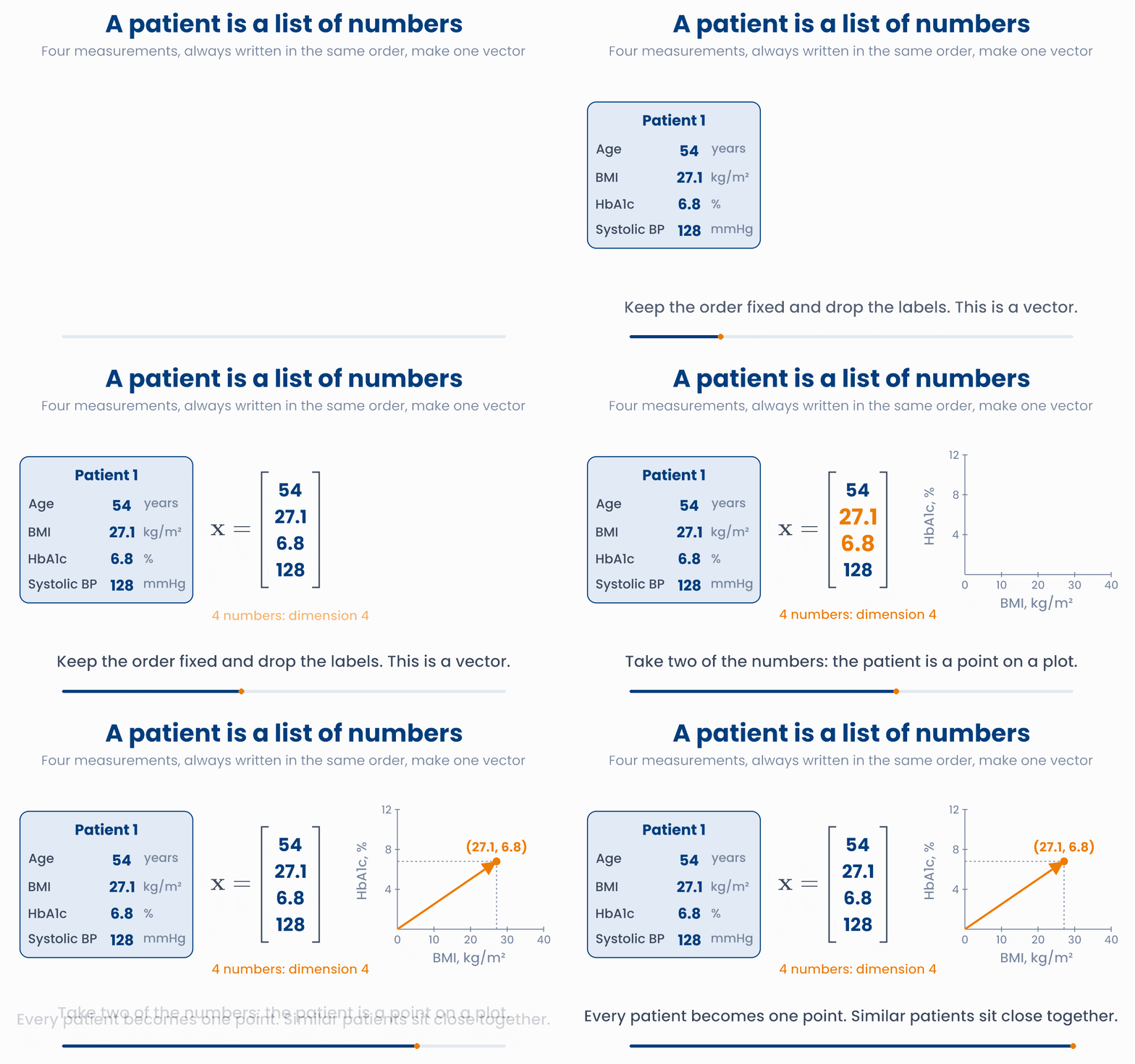
We write a vector with a bold small letter, \(\mathbf{x}\). It is often written as a column:
- Each number in the vector is a component (or an element). \(x_3 = 6.8\) is the third component: the HbA1c.
- The number of components is the dimension of the vector. This vector has dimension 4. We usually call it \(p\), for the number of measurements.
- In machine learning, each measurement is called a feature. So a patient is a feature vector.
Here the subscript counts measurements, not patients. When we need both, we use two subscripts, \(x_{ij}\), as in Lesson 1.1. That comes back at the end of this lesson.
A vector also has a picture. Take just two features, BMI and HbA1c. Then a patient is a point on a plot, or an arrow from zero to that point. The two components are how far to go across and how far to go up.
A patient is a point, or an arrow
Drag the orange point. The arrow, its two components and the readout follow. The pale dots are four other patients from the same clinic.
With two features we can draw the picture. With four features the patient is a point in a four-dimensional space. Nobody can draw that, but the arithmetic is exactly the same. A tumour sample with 20,000 measured genes is a point in a space with 20,000 dimensions.
Why you will care later
import numpy as np
x = np.array([54, 27.1, 6.8, 128])   # age, BMI, HbA1c, SBP
print(x[2])     # 6.8   the HbA1c: x_3 in maths, x[2] in Python
print(len(x)) # 4 the dimensionEach patient in a study has 20 laboratory values and 3 vital signs recorded. What is the dimension of one patient's vector?
3 Adding and scaling vectors
A patient starts a new blood pressure drug. At the first visit (baseline) their systolic and diastolic pressures are 150 and 95 mmHg. Six months later they are 132 and 83 mmHg. Each visit is a vector of dimension 2: \(\mathbf{b} = (150, 95)\) and \(\mathbf{f} = (132, 83)\).
How much did the patient change? Subtract the vectors component by component: the first from the first, the second from the second.
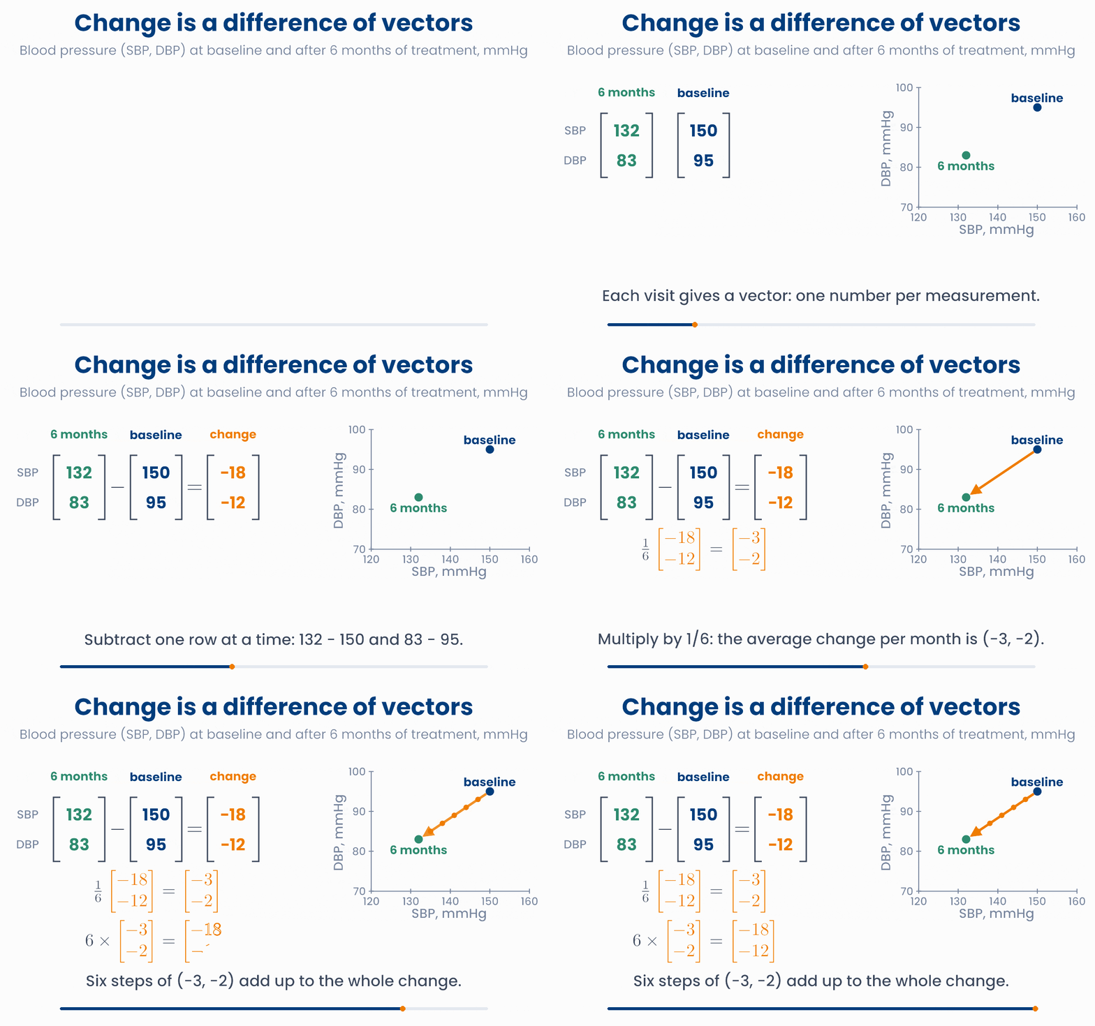
On the plot, the change vector is the arrow from the baseline point to the follow-up point. Adding works the same way, component by component. If you add the change to the baseline, you arrive at the follow-up: \(\mathbf{b} + (\mathbf{f} - \mathbf{b}) = \mathbf{f}\).
You can also multiply a vector by a single number. A single number is called a scalar. Multiplying by a scalar is called scaling, and it multiplies every component by that number. For example, the average change per month is the change divided by 6:
The arrow keeps its direction and becomes 6 times shorter. Scaling by a negative number turns the arrow round to point the other way.
Baseline plus a scaled change
Drag the blue (baseline) or green (6 months) point. The orange arrow is the change f − b. Move the slider: the purple ring shows where the patient would be after t months if the change went on at the same steady rate.
Scaling also describes a change of units. A glucose tolerance test gives three glucose readings, at 0, 1 and 2 hours: \((5.0, 9.0, 7.0)\) mmol/L. To convert mmol/L to mg/dL you multiply by 18. So the same results in mg/dL are \(18 \times (5.0, 9.0, 7.0) = (90, 162, 126)\).
A preview: standardising
import numpy as np
baseline = np.array([150, 95])    # SBP, DBP in mmHg
followup = np.array([132, 83])
change = followup - baseline
print(change)         # [-18 -12]
print(change / 6)     # [-3. -2.]   average change per month
glucose = np.array([5.0, 9.0, 7.0])   # mmol/L at 0, 1 and 2 hours
print(glucose * 18)   # [ 90. 162. 126.]   the same results in mg/dL
Common mistake
A patient's HbA1c (%) and fasting glucose (mmol/L) are \((8.0, 9.5)\) at baseline and \((7.2, 8.1)\) after 3 months. What is the change vector, follow-up minus baseline?
4 The dot product: a weighted sum
Many clinical risk scores are built in the same way. Each measurement gets a weight. You multiply each measurement by its weight, and you add up the results. A large weight means that measurement matters a lot for the score.
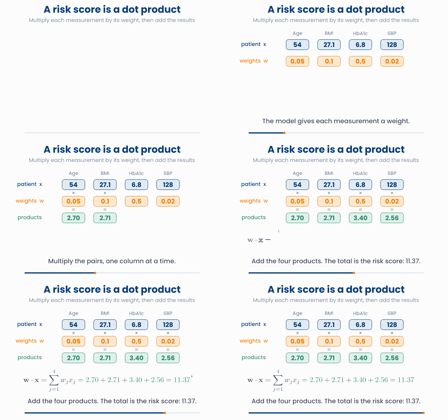
This operation has a name: the dot product of the weight vector \(\mathbf{w}\) and the patient vector \(\mathbf{x}\). Multiply the pairs, then add them up. The result is one number, not a vector.
This is the sigma from Lesson 1.1. The only new part is that each term is a product of two numbers.
Patient 1 with the weights in the animation
- Age: \(0.05 \times 54 = 2.70\)
- BMI: \(0.1 \times 27.1 = 2.71\)
- HbA1c: \(0.5 \times 6.8 = 3.40\)
- Systolic BP: \(0.02 \times 128 = 2.56\)
- Add them: \(\mathbf{w}\cdot\mathbf{x} = 2.70 + 2.71 + 3.40 + 2.56 = 11.37\)
The weights here are made up to show the arithmetic. In a real model, the weights are learned from data.
A risk score is multiply-then-add
Pick a patient and move the weights. The orange cell is the product that adds most to the score. Try a negative weight: that measurement now lowers the score.
Notice that the weight for systolic BP is small (0.02) but its product is not small, because blood pressures are large numbers. The size of a weight always depends on the units of its feature.
Why you will care later
import numpy as np
x = np.array([54, 27.1, 6.8, 128])     # age, BMI, HbA1c, SBP
w = np.array([0.05, 0.1, 0.5, 0.02])   # weights
print(w * x)              # [2.7  2.71 3.4  2.56]   the four products
print(np.sum(w * x))      # 11.370000000000001   then add them up
print(w @ x)              # 11.370000000000001   @ does both steps: the dot product
Computers store most decimals with a tiny rounding error, so Python prints 11.370000000000001. For any practical purpose that is 11.37.
A heart-risk score uses the features (current smoker, hours of exercise per week, LDL cholesterol in mmol/L) with weights \(\mathbf{w} = (2, -0.5, 1)\). A patient has \(\mathbf{x} = (1, 4, 3.0)\). What is \(\mathbf{w}\cdot\mathbf{x}\)?
5 Length and distance
How similar are two patients? One simple answer: draw them as points and measure the straight line between them. Short line, similar patients.
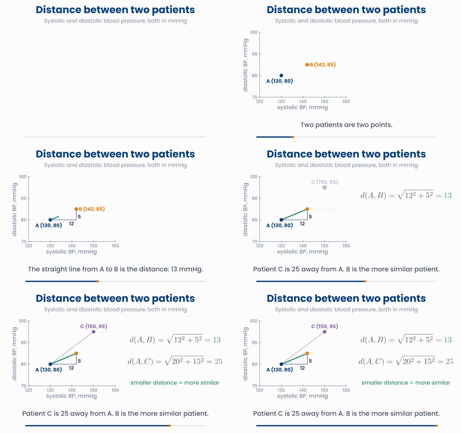
The straight line is the long side of a right-angled triangle, so Pythagoras gives its length: square each difference, add the squares, take the square root. For patients A and B, the differences are 12 and 5 mmHg, and \(\sqrt{12^2 + 5^2} = \sqrt{169} = 13\) mmHg.
The length (or norm) of a vector uses the same rule. It is written with double bars:
The Euclidean distance between two patients \(\mathbf{a}\) and \(\mathbf{b}\) is the length of their difference vector. It works for any number of features: with 20 features, there are 20 squared differences under the root.
Distance is the basis of two common methods. k-nearest neighbours predicts for a new patient from the \(k\) most similar patients in the data, the ones at the smallest distance. Clustering groups patients that sit close together, for example to find subtypes of a disease.
There is a trap. Every feature has its own units, and the distance simply adds up the squared differences. A feature measured in big numbers can swamp the others.
Who is the nearest neighbour? It depends on the units
A, B and C are patients. The green line joins A to its nearest neighbour. Switch the glucose units and watch which patient is nearest to A. Drag any patient to try other values. The plot keeps one unit across equal to one unit up, so the lines show the true distances.
Nothing about the patients changed when you switched units, yet the "most similar" patient did. In mmol/L, patient B looks most like A, even though B's fasting glucose (7.5 mmol/L) is in the diabetes range and A's (5.5) is normal. After standardising, C is nearest: same glucose as A, ten years older.
Standardise before you measure distance
import numpy as np
a = np.array([130, 80])     # patient A: SBP, DBP in mmHg
b = np.array([142, 85])     # patient B
print(b - a)                         # [12  5]
print(np.sqrt(np.sum((b - a)**2)))   # 13.0   square, add, square root
print(np.linalg.norm(b - a))         # 13.0   the same in one step
Why you will care later
Patient P has blood pressure (SBP, DBP) = (120, 80) mmHg and patient Q has (126, 88) mmHg. What is the Euclidean distance between them?
5.1 Cosine similarity: same pattern, different level
Sometimes the overall size of a vector is not what you care about. Two tumour samples are sequenced. Sample 2 was sequenced more deeply, so every gene has twice the count of sample 1: \((2, 4, 6)\) and \((4, 8, 12)\) for three genes. The pattern of expression is identical, but the Euclidean distance between them is \(\sqrt{2^2 + 4^2 + 6^2} \approx 7.48\), which is large.
Picture the two vectors as arrows. Scaling a vector changes its length but not its direction. So compare the directions instead. The cosine similarity is the cosine of the angle \(\theta\) between the two arrows:
- \(\cos\theta = 1\): the arrows point the same way. Same pattern, whatever the overall level.
- \(\cos\theta = 0\): the arrows are at a right angle. The patterns are unrelated.
- \(\cos\theta = -1\): the arrows point in opposite directions. (This needs negative values, such as gene expression measured above or below average.)
Direction versus length
Drag the tip of either arrow. Then press Double or Halve: sample 2 gets longer or shorter, the distance changes, but the angle and the cosine similarity stay the same.
For the two tumour samples: \(\mathbf{a}\cdot\mathbf{b} = 2\times4 + 4\times8 + 6\times12 = 112\), \(\lVert\mathbf{a}\rVert = \sqrt{56}\) and \(\lVert\mathbf{b}\rVert = \sqrt{224}\). So \(\cos\theta = 112 / \sqrt{56 \times 224} = 112/112 = 1\). Same direction: same pattern.
import numpy as np
s1 = np.array([2, 4, 6])      # expression of three genes, sample 1
s2 = np.array([4, 8, 12])     # sample 2: same pattern, twice the level
print(np.linalg.norm(s2 - s1).round(2))   # 7.48   far apart by distance
cos = s1 @ s2 / (np.linalg.norm(s1) * np.linalg.norm(s2))
print(cos) # 1.0 but pointing the same wayTwo blood samples have the same pattern of gene expression, but sample 2 was sequenced more deeply, so every count is twice as high. Which measure says the two samples are alike?
6 The data matrix
Now stack the patient vectors on top of each other, one row per patient. The result is a rectangular table of numbers: a matrix. We name matrices with a capital letter, usually \(X\) for the data.
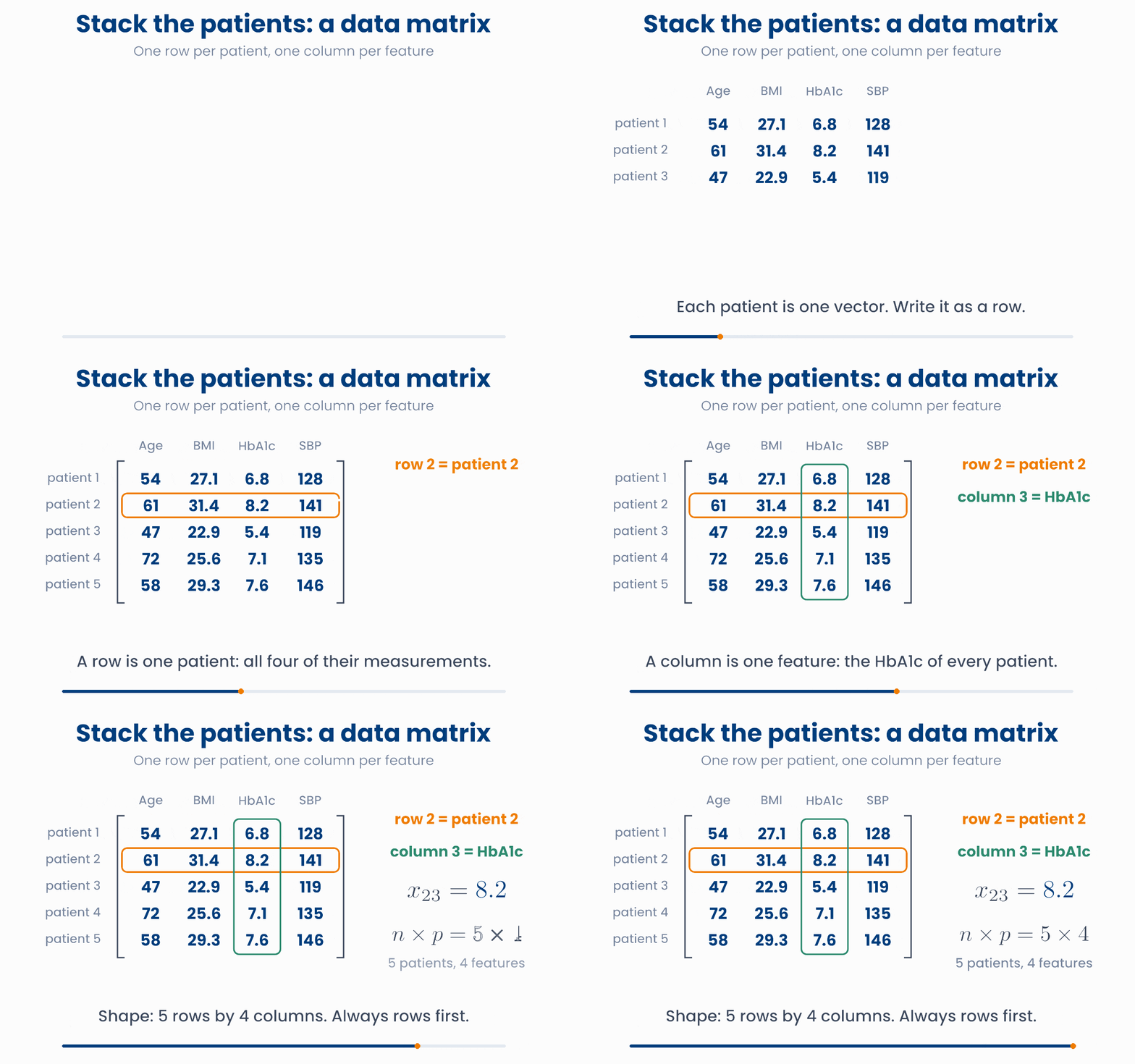
- Each row is one patient: their whole feature vector.
- Each column is one feature: its values for every patient. A column is also a vector, of length \(n\).
- The shape of the matrix is "rows by columns", \(n \times p\): \(n\) patients and \(p\) features. Always rows first.
- One entry is \(x_{ij}\): patient \(i\), feature \(j\). This is the two-subscript notation from Lesson 1.1.
A row is a patient, a column is a feature
Choose row or column, then move the slider. A row gives you one patient's vector. A column gives you one feature for every patient, and you can take its mean.
Real data matrices are big. A hospital cohort might have \(n = 50{,}000\) patients and \(p = 30\) features. A gene-expression study often has the opposite shape: \(n = 200\) tumour samples and \(p = 20{,}000\) genes. When there are far more features than patients, many classical methods break down. That is a central problem in precision medicine, and Lesson 2.2 shows one way to deal with it.
import numpy as np
X = np.array([[54, 27.1, 6.8, 128],
              [61, 31.4, 8.2, 141],
              [47, 22.9, 5.4, 119],
              [72, 25.6, 7.1, 135],
              [58, 29.3, 7.6, 146]])   # rows: patients, columns: age, BMI, HbA1c, SBP
print(X.shape)         # (5, 4)   n = 5 patients, p = 4 features
print(X[1, 2])         # 8.2      x_23: Python counts rows and columns from 0
print(X[:, 2].mean().round(2))  # 7.02   the mean of column 3, HbA1c
Why you will care later
model.fit(X, y). \(X\) is exactly this matrix, with shape (patients, features). Getting your data into this shape is the first step of every analysis.A study measures 20,000 genes in 150 tumour samples. The data are stored with one row per sample. What is the shape of the data matrix?
7 Check your understanding
Five short questions on this lesson. Nothing is graded or saved outside this browser. If you choose a wrong option you get a hint, and you can try again.
Clinic A stores a patient as (age, HbA1c, SBP) = (61, 8.2, 141). Clinic B stores the same patient as (141, 61, 8.2). What is true?
A score uses the weights \(\mathbf{w} = (0.04, 0.3, 0.01)\) for (age, HbA1c, SBP). A patient has \(\mathbf{x} = (50, 7.0, 130)\). What is the score \(\mathbf{w}\cdot\mathbf{x}\)?
You find each patient's nearest neighbours using age (years) and serum creatinine. Then creatinine is changed from mg/dL to µmol/L, which multiplies every creatinine value by 88.4. What happens?
Two blood samples have expression profiles \((10, 20, 5)\) and \((30, 60, 15)\) for three genes. Which statement is true?
A data matrix \(X\) has shape \(300 \times 12\). What does row 7 hold?