

1 Introduction
A doctor gives a child paracetamol. The usual dose is 15 mg for each kilogram of body weight. That sentence is a function: a rule that takes one number in (the weight) and gives exactly one number back (the dose).
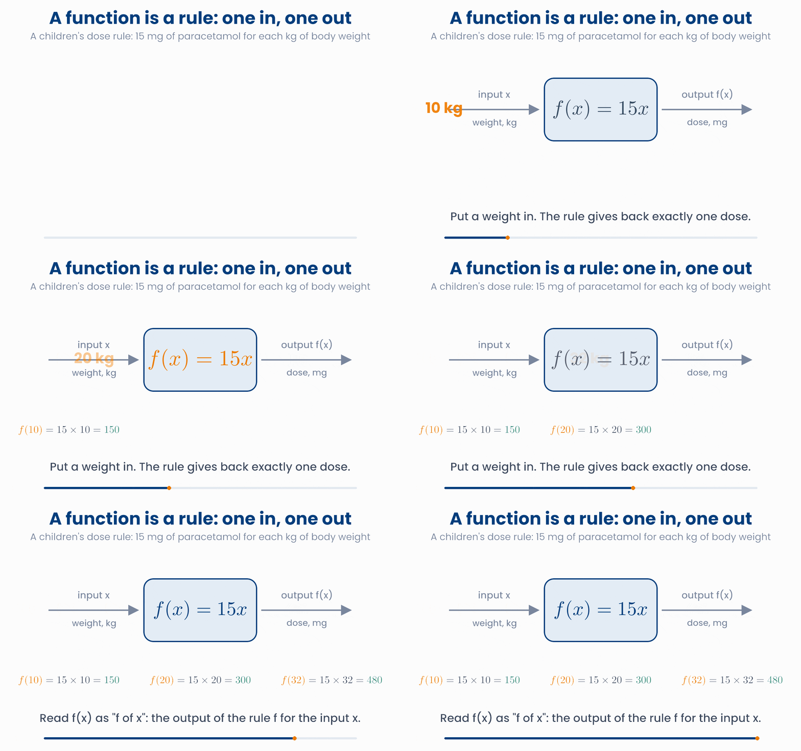
We write the rule as
- \(x\) is the input: here, the weight in kg.
- \(f(x)\) is the output: the dose in mg that the rule gives for that weight.
- \(f(20) = 15 \times 20 = 300\) means "for a 20 kg child, the rule gives 300 mg".
A function does not have to be one neat formula. Real dosing rules have a maximum. For paracetamol, the dose for one time is not usually more than 1,000 mg, however heavy the patient. The rule is still a function, because each weight still gives exactly one dose.
A dosing rule is a function
Move the weight. The dot shows the dose the rule gives. Watch what happens above about 67 kg.
Most models in statistics and machine learning are built from a small set of functions. This lesson covers the ones you will meet again and again:
- straight lines, for steady change;
- exponentials, for growth and decay, such as a drug leaving the blood;
- logarithms, for values that range over many tenfolds, such as viral load or gene expression;
- odds and the sigmoid, for turning a risk score into a probability.
def dose(weight_kg):
    return min(15 * weight_kg, 1000)   # 15 mg/kg, at most 1,000 mg

print(dose(20))   # 300
print(dose(80)) # 10002 Straight lines
On average, systolic blood pressure rises steadily with age in adults. A steady change is drawn as a straight line. Every straight line has the same form:
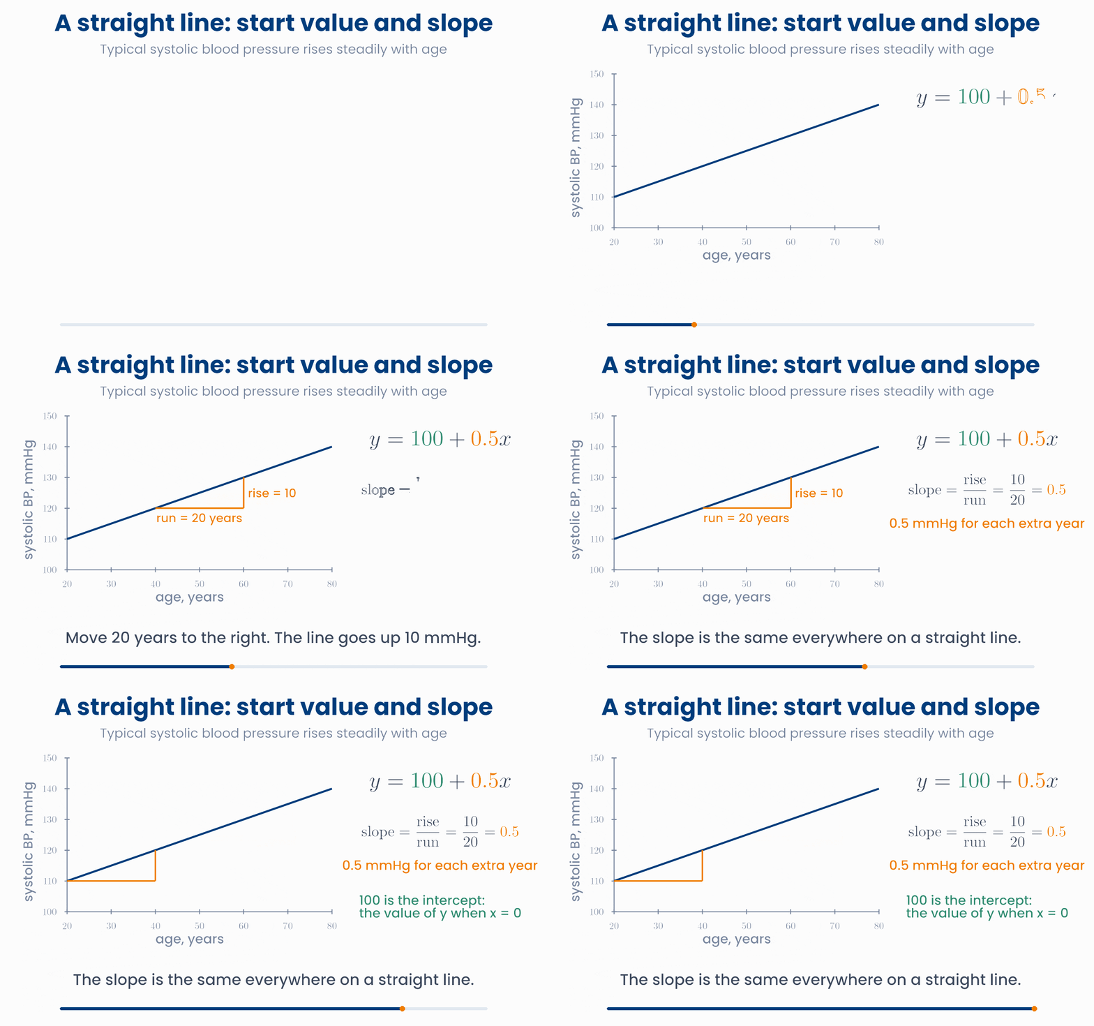
- The slope \(m\) is how much \(y\) changes when \(x\) goes up by 1. It is "rise over run". In the animation, \(m = 0.5\): blood pressure goes up 0.5 mmHg for each extra year of age.
- The intercept \(c\) is the value of \(y\) when \(x = 0\). It is where the line crosses the vertical axis.
- A positive slope goes up to the right. A negative slope goes down. A slope of 0 is flat: \(x\) makes no difference to \(y\).
Move a line through the patients
Each dot is a patient. Change the intercept and the slope until the line runs through the middle of the cloud.
Why you will care later
import numpy as np
age = np.array([30, 45, 60, 75])
sbp = 100 + 0.5 * age      # the line, applied to every patient at once
print(sbp) # [115. 122.5 130. 137.5]A model says: eGFR (kidney function, mL/min) \( = 120 - 0.8 \times \text{age}\). What does the number \(-0.8\) tell you?
2.1 When a line is not enough
Some relationships bend. The risk of death is higher for people who are very underweight and for people who are very overweight. A straight line can only go up or down, so it cannot show this U shape. Adding a squared term lets the line bend:
A function made of powers of \(x\) like this is a polynomial. Its degree is the highest power: 1 for a line, 2 for a single bend, 3 for an S-like curve with two bends.
Can the curve follow the data?
The dots show an illustrative U-shaped link between BMI and the relative risk of death. Choose the degree of the polynomial and watch how well it follows the dots.
More bends is not always better
3 Exponential growth and decay
After a dose, many drugs leave the blood in a special way: in each hour, the body removes the same fraction of what is left, not the same amount. When a fixed fraction goes each time, the result is exponential decay.
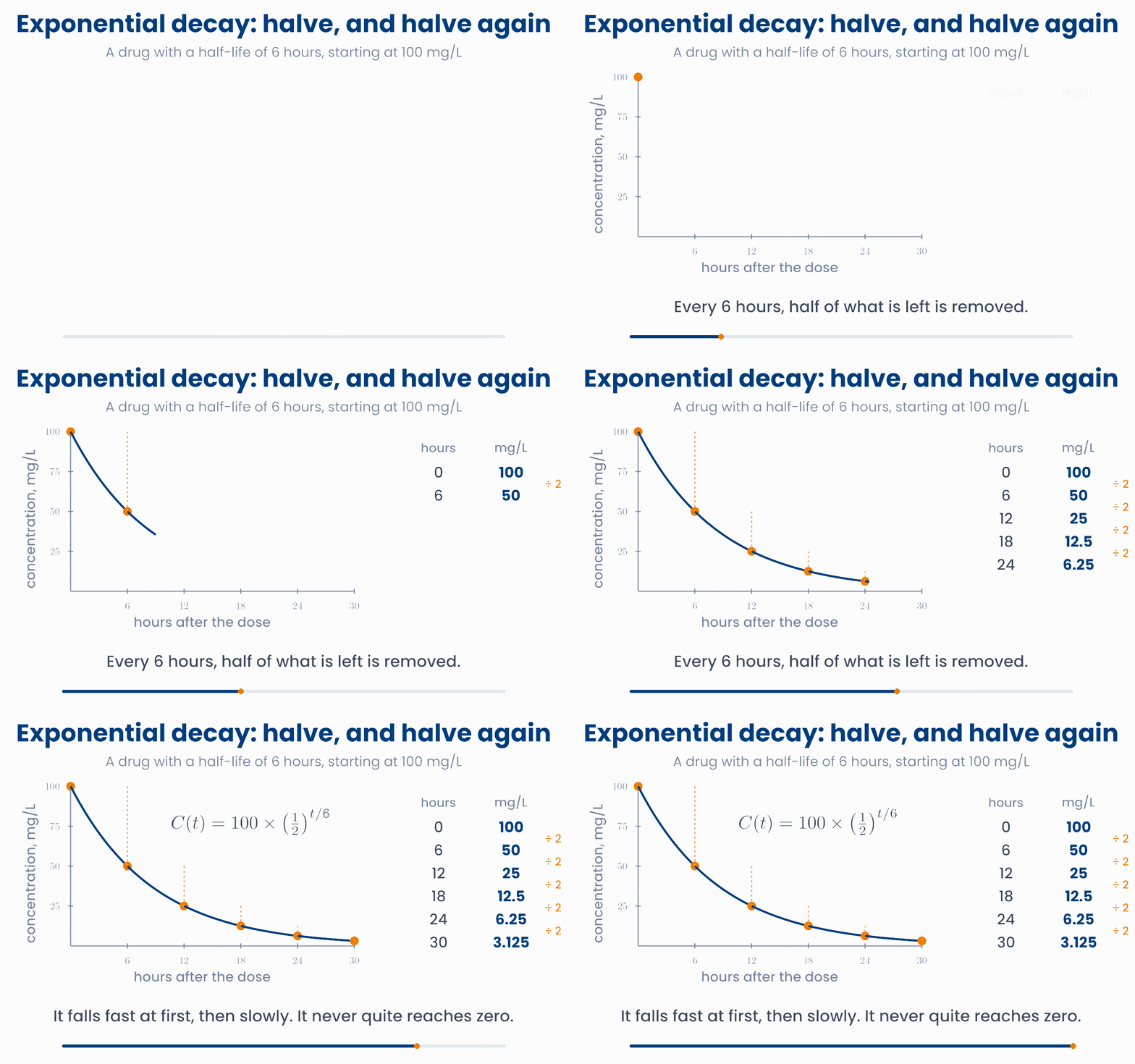
The time it takes for the amount to halve is the half-life, \(T\). After one half-life 50% is left, after two 25%, after three 12.5%, and so on:
You will often see the same curve written with the number \(e \approx 2.718\), which is the natural base for growth and decay:
Growth works the same way, with a plus sign. Bacteria that divide every 20 minutes double in number every 20 minutes. A tumour can have a doubling time of a few months. Growth that doubles at a steady rate is exponential growth.
Change the half-life
Move the half-life slider and watch how fast the drug is cleared. Then tick the log scale box: the curve becomes a straight line.
Straight on a log scale
import numpy as np
t = np.array([0, 6, 12, 24])         # hours
k = np.log(2) / 6                    # half-life of 6 hours
print(np.round(100 * np.exp(-k * t), 2)) # [100. 50. 25. 6.25]An antibiotic has a half-life of 2 hours. About what fraction of a dose is still in the blood after 8 hours?
4 Logarithms and log scales
A logarithm answers one question: how many times do I multiply the base to get this number?
- \(\log_{10}(1000) = 3\), because \(10 \times 10 \times 10 = 1000\).
- \(\log_{2}(8) = 3\), because \(2 \times 2 \times 2 = 8\).
- \(\ln(x)\) is the natural log, with base \(e \approx 2.718\). It is the default in most statistics software, including
np.log.
So a logarithm counts multiplications. This makes it the right tool for numbers that range over many tenfolds. An HIV viral load can be 1,000,000 copies/mL before treatment and below 50 a few months later.
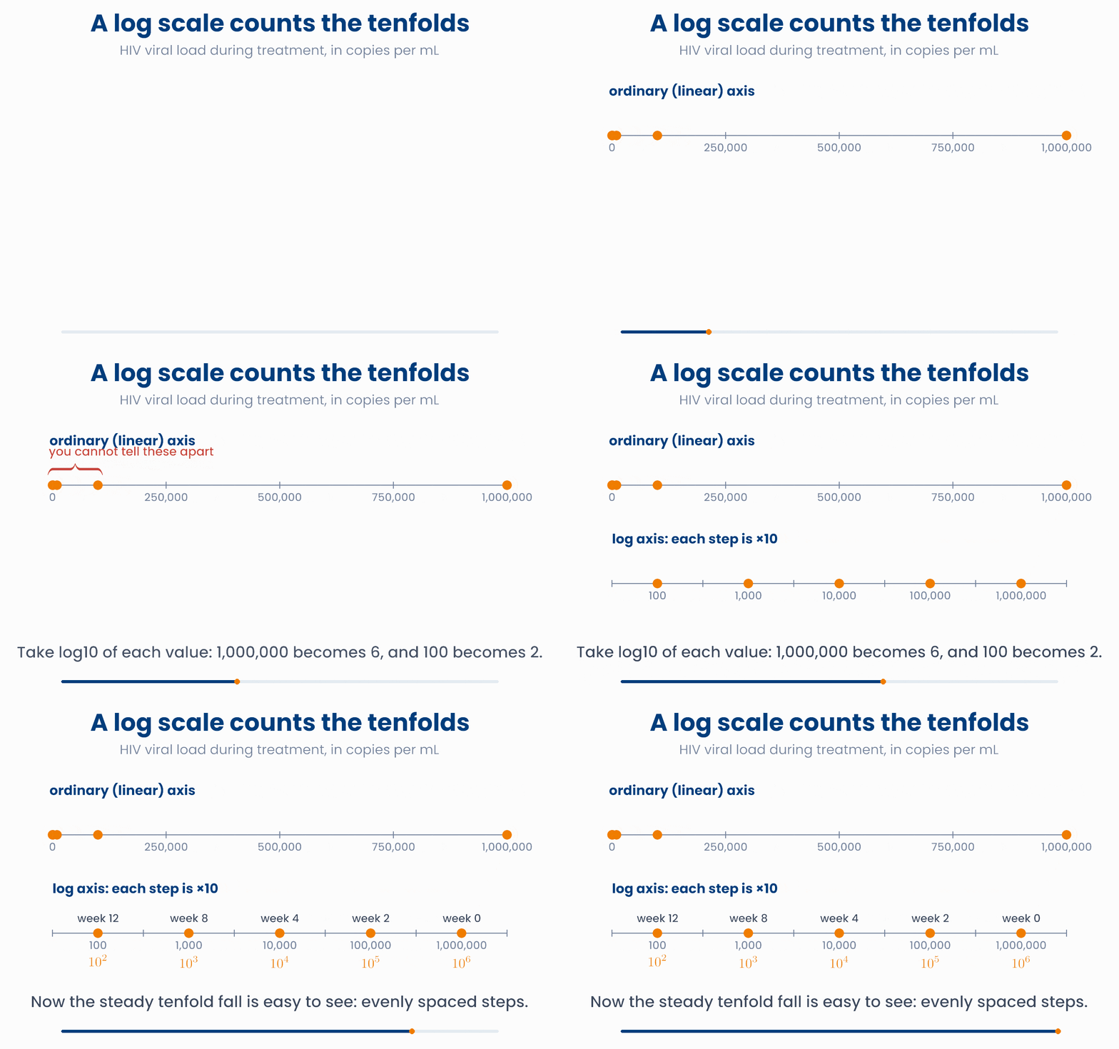
The logarithm has one property that makes it very useful in statistics: it turns multiplying into adding.
In genomics, a change in gene expression is reported as a log2 fold change. A fold change is a ratio: treated divided by control. Its log2 is +1 when expression doubles and −1 when it halves.
Why gene expression uses log2 fold change
Move the slider to change how much a gene goes up or down after treatment. Compare where the gene lands on the two scales.
On the ratio scale, every "down" change is squeezed between 0 and 1, while "up" changes can stretch out to any size. A gene that falls 4 times (ratio 0.25) looks much smaller than a gene that rises 4 times (ratio 4). On the log2 scale they are mirror images, \(-2\) and \(+2\), which is fair.
Why you will care later
import numpy as np
print(np.log10([100, 1000, 1_000_000]))   # [2. 3. 6.]
print(np.log2(400 / 100))                 # 2.0   expression up 4 times
print(np.log2(25 / 100))                  # -2.0  expression down 4 times
print(np.log(np.e)) # 1.0 np.log is the natural logA patient's viral load falls from 100,000 to 1,000 copies/mL. What is the change on a \(\log_{10}\) scale?
5 Odds and log-odds
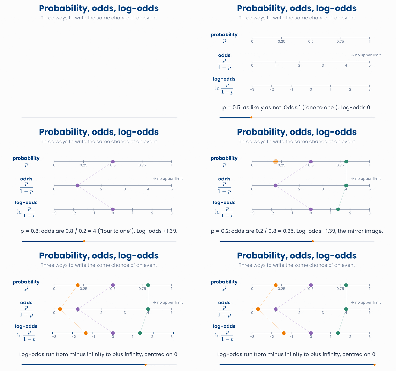
A probability \(p\) is a chance between 0 and 1. If 80% of patients respond to a drug, \(p = 0.8\). Medicine also uses another way to say the same thing, the odds:
For \(p = 0.8\), the odds are \(0.8 / 0.2 = 4\): responders outnumber non-responders four to one. The log-odds (also called the logit) is the natural log of the odds.
| Scale | Range | "As likely as not" |
|---|---|---|
| Probability \(p\) | 0 to 1 | 0.5 |
| Odds \(p/(1-p)\) | 0 to infinity | 1 |
| Log-odds \(\ln\frac{p}{1-p}\) | minus infinity to plus infinity | 0 |
Turn a probability into odds and log-odds
Move the probability. Notice that the log-odds is 0 at p = 0.5, and is symmetric: p = 0.2 and p = 0.8 give the same number with opposite signs.
Why you will care later
import numpy as np
p = np.array([0.2, 0.5, 0.8])
odds = p / (1 - p)
print(odds)                   # [0.25 1.   4.  ]
print(np.round(np.log(odds), 2)) # [-1.39 0. 1.39]In a trial, 25% of patients have a side effect. What are the odds of the side effect?
6 The sigmoid: from score to probability
Many models first add up a score from a patient's measurements, for example \(z = -9 + 1.5 \times \text{glucose}\). The score can be any number, but a risk must lie between 0 and 1. The sigmoid (or logistic) function does the conversion:
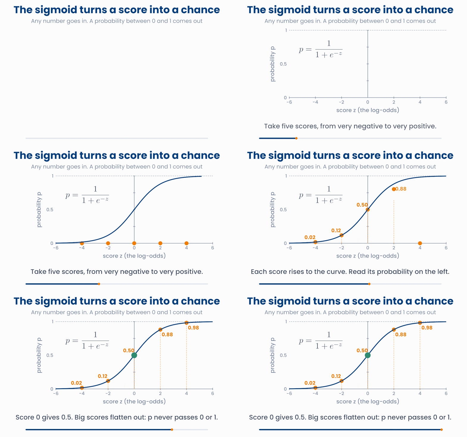
- A score of 0 gives \(p = 0.5\).
- Large positive scores give probabilities close to 1. Large negative scores give probabilities close to 0.
- The curve is steepest in the middle. There, a small change in the score changes the risk a lot. Far out on either side, the risk hardly moves.
A risk model for one biomarker
Each dot is a patient: at the top if they have the disease, at the bottom if not. Change the two numbers in the score and fit the S-curve to the patients.
This is the whole idea of logistic regression, in one picture: a straight-line score, passed through the sigmoid, gives a probability. The intercept \(\beta_0\) moves the S-curve left and right. The slope \(\beta_1\) makes it steeper or flatter.
Key idea
import numpy as np
def sigmoid(z):
    return 1 / (1 + np.exp(-z))

z = np.array([-4, -2, 0, 2, 4])
print(np.round(sigmoid(z), 2))    # [0.02 0.12 0.5  0.88 0.98]

glucose = 7.0
print(round(sigmoid(-9 + 1.5 * glucose), 2))   # 0.82
Why you will care later
7 Check your understanding
Five short questions on this lesson. Nothing is graded or saved outside this browser. If you choose a wrong option you get a hint, and you can try again.
A model says HbA1c (%) \( = 5.2 + 0.03 \times \text{weight (kg)}\). What does it predict for a patient who weighs 80 kg?
A drug has a half-life of 12 hours. Starting from 80 mg/L, what is the concentration after 36 hours?
A gene has a log2 fold change of \(-3\) after treatment. What happened to its expression?
Why do models such as logistic regression put a straight line on the log-odds scale rather than on the probability scale?
A risk score for a patient is \(z = 0\). What risk does the sigmoid give?